The same plot in 14 other libraries — Python: Altair, Bokeh, lets-plot, Matplotlib, Plotly, Pygal, Seaborn; R: ggplot2; Julia: Makie.jl; JavaScript: Chart.js, D3.js, Apache ECharts, Highcharts, MUI X Charts. Compare all 15 side by side: Tanabe-Sugano Diagram for Crystal Field Theory in Python, R, Julia and JavaScript.
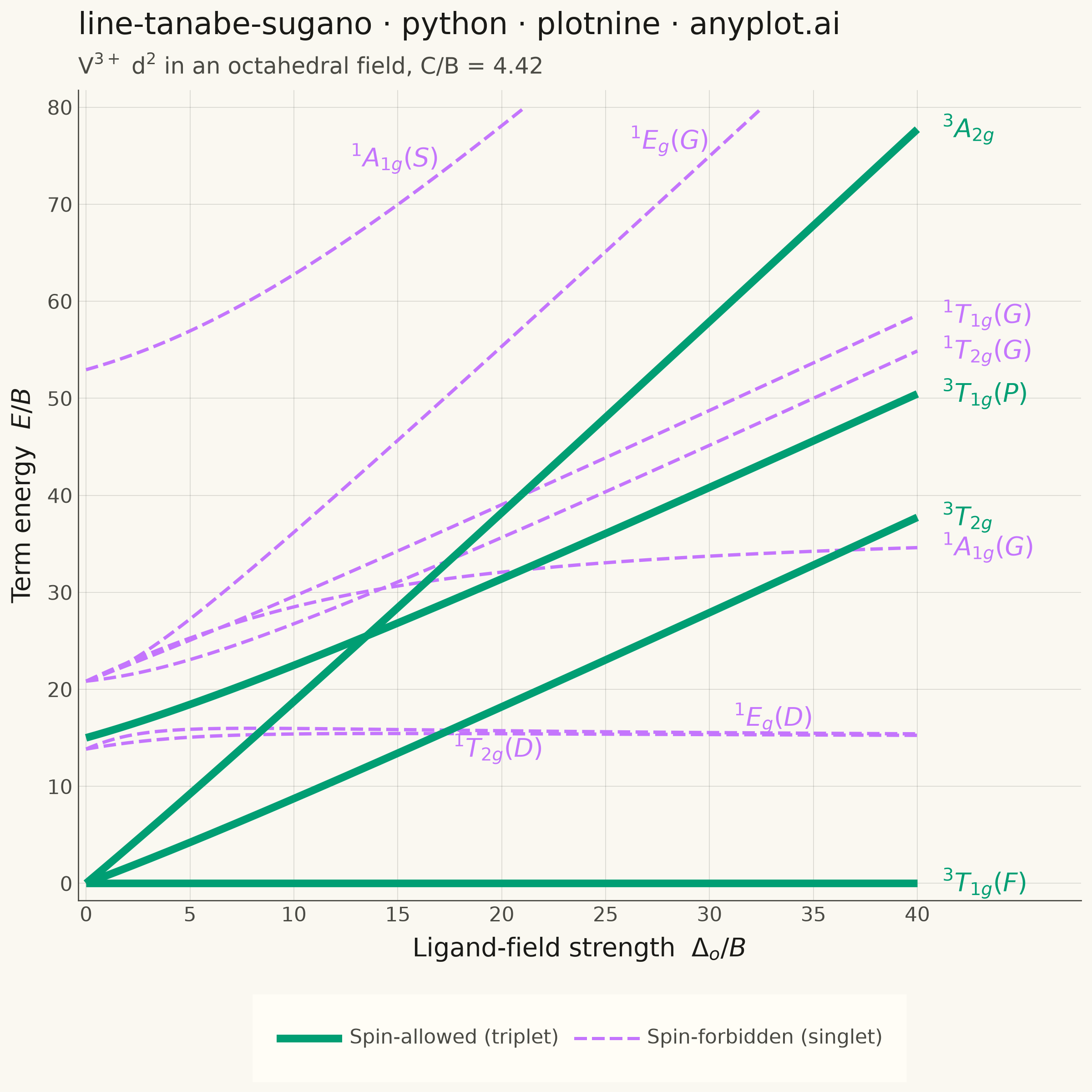
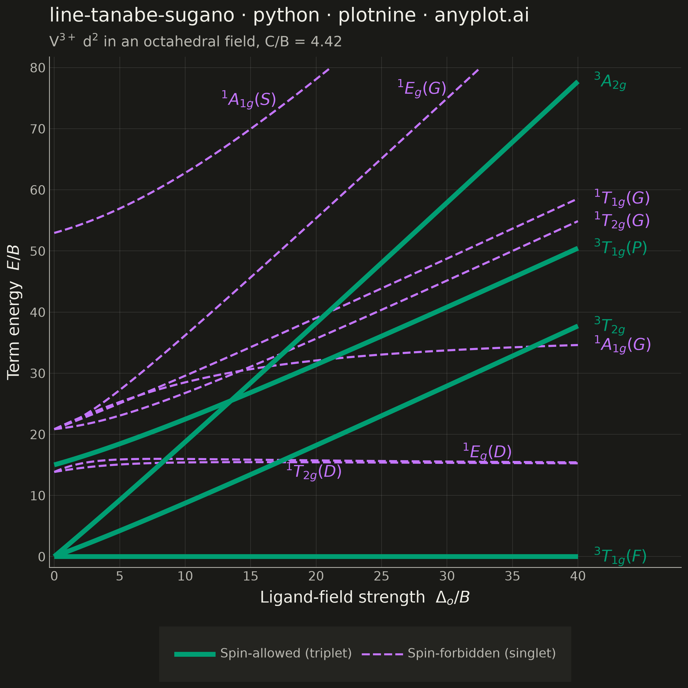
A Tanabe-Sugano diagram plots the energies of the electronic term states of a transition-metal ion in an octahedral ligand field as continuous functions of the field strength. The x-axis is the reduced ligand-field strength Δ_o/B (octahedral splitting divided by the Racah parameter B) and the y-axis is the reduced term energy E/B measured from the ground term, which therefore runs along the x-axis itself as a horizontal line at E/B = 0. Each term — labeled with its full symbol including spin multiplicity and Mulliken label — is one curve, and for d⁴–d⁷ a vertical line marks the high-spin/low-spin crossover where the ground term changes and every curve kinks. Chemists read the chart in reverse: matching ratios of observed UV-Vis band energies against the curves yields both Δ_o and B for a real complex.
""" anyplot.ai
line-tanabe-sugano: Tanabe-Sugano Diagram for Crystal Field Theory
Library: plotnine 0.15.8 | Python 3.13.15
Quality: 90/100 | Created: 2026-10-01
"""

import os

import numpy as np
import pandas as pd
from plotnine import (
    aes,
    element_blank,
    element_line,
    element_rect,
    element_text,
    geom_line,
    geom_text,
    ggplot,
    labs,
    scale_color_manual,
    scale_linetype_manual,
    scale_size_manual,
    scale_x_continuous,
    scale_y_continuous,
    theme,
    theme_minimal,
)


# Theme tokens (Imprint palette + theme-adaptive chrome)
THEME = os.getenv("ANYPLOT_THEME", "light")
PAGE_BG = "#FAF8F1" if THEME == "light" else "#1A1A17"
ELEVATED_BG = "#FFFDF6" if THEME == "light" else "#242420"
INK = "#1A1A17" if THEME == "light" else "#F0EFE8"
INK_SOFT = "#4A4A44" if THEME == "light" else "#B8B7B0"
SPIN_ALLOWED = "#009E73"  # Imprint palette position 1 — always the first series
SPIN_FORBIDDEN = "#C475FD"  # Imprint palette position 2

# Data — d2 (V3+) term energies from the Tanabe-Sugano matrices, in units of the
# Racah parameter B at C/B = 4.42, with Dq = (delta_o / B) / 10
c_over_b = 4.42
delta_over_b = np.linspace(0, 40, 321)
dq = delta_over_b / 10.0
ground_term = r"$^{3}T_{1g}(F)$"

# A symmetry that occurs once in the d2 configuration is a single state, so its
# energy is linear in the ligand-field strength
energies = {r"$^{3}T_{2g}$": -8 + 2 * dq, r"$^{3}A_{2g}$": -8 + 12 * dq, r"$^{1}T_{1g}(G)$": 4 + 2 * c_over_b + 2 * dq}

# A symmetry that occurs twice gives a 2x2 matrix (diagonal, off-diagonal mixing,
# diagonal); diagonalizing it keeps the two roots an avoided crossing instead of
# letting the curves touch and swap identity
blocks = {
    (r"$^{3}T_{1g}(F)$", r"$^{3}T_{1g}(P)$"): (-5 - 8 * dq, -6.0, 4 + 2 * dq),
    (r"$^{1}E_{g}(D)$", r"$^{1}E_{g}(G)$"): (1 + 2 * c_over_b - 8 * dq, 2 * np.sqrt(3), 2 * c_over_b + 12 * dq),
    (r"$^{1}T_{2g}(D)$", r"$^{1}T_{2g}(G)$"): (1 + 2 * c_over_b - 8 * dq, 2 * np.sqrt(3), 2 * c_over_b + 2 * dq),
    (r"$^{1}A_{1g}(G)$", r"$^{1}A_{1g}(S)$"): (
        10 + 5 * c_over_b - 8 * dq,
        np.sqrt(6) * (2 + c_over_b),
        8 + 4 * c_over_b + 12 * dq,
    ),
}
for (lower_term, upper_term), (first, mixing, second) in blocks.items():
    block = np.zeros((len(dq), 2, 2))
    block[:, 0, 0] = first
    block[:, 1, 1] = second
    block[:, 0, 1] = block[:, 1, 0] = mixing
    energies[lower_term], energies[upper_term] = np.linalg.eigvalsh(block).T

# Every energy is measured from the ground term, which is flat at E/B = 0 by
# construction; the upper partners of the avoided crossings keep climbing past
# the top of the window, so they are clipped where they leave the frame
terms = pd.DataFrame(energies, index=delta_over_b)
terms = terms.sub(terms[ground_term], axis=0)

df = terms.stack().reset_index()
df.columns = ["delta_over_b", "term", "energy_over_b"]
df = df[df["energy_over_b"] <= 80]
df["spin"] = pd.Categorical(
    np.where(df["term"].str.startswith("$^{3}"), "Spin-allowed (triplet)", "Spin-forbidden (singlet)"),
    categories=["Spin-allowed (triplet)", "Spin-forbidden (singlet)"],
    ordered=True,
)

# Term labels sit in a gutter right of the curves, each at its own end value. The
# two 1D-derived terms stay near-coincident all the way across and the two upper
# partners leave the window, so those four are labelled along the curve instead,
# each resting on the line it names — above it for the upper term of a pair,
# below it for the lower one
along_curve = {r"$^{1}E_{g}(D)$": 35.0, r"$^{1}T_{2g}(D)$": 22.0, r"$^{1}E_{g}(G)$": 30.0, r"$^{1}A_{1g}(S)$": 17.0}
anchors = pd.DataFrame(
    [
        {
            "delta_over_b": x,
            "term": term,
            "energy_over_b": terms[term].to_numpy()[np.searchsorted(delta_over_b, x)],
            "spin": "Spin-forbidden (singlet)",  # all four along-curve terms are singlets
        }
        for term, x in along_curve.items()
    ]
)
lower_of_pair = anchors["term"] == r"$^{1}T_{2g}(D)$"

curve_ends = df[(df["delta_over_b"] == delta_over_b[-1]) & ~df["term"].isin(along_curve)].copy()
curve_ends["delta_over_b"] = 41.2

# Plot
plot = (
    ggplot(df, aes("delta_over_b", "energy_over_b", group="term", color="spin"))
    + geom_line(aes(linetype="spin", size="spin"))
    + geom_text(aes(label="term"), data=curve_ends, size=10, ha="left", show_legend=False)
    + geom_text(aes(label="term"), data=anchors[~lower_of_pair], size=10, ha="right", va="bottom", show_legend=False)
    + geom_text(aes(label="term"), data=anchors[lower_of_pair], size=10, ha="right", va="top", show_legend=False)
    + scale_color_manual(values=[SPIN_ALLOWED, SPIN_FORBIDDEN])
    + scale_linetype_manual(values=["solid", "dashed"])
    + scale_size_manual(values=[1.7, 0.75])
    + scale_x_continuous(limits=(0, 47.5), breaks=range(0, 41, 5), expand=(0.008, 0))
    + scale_y_continuous(limits=(0, 80), breaks=range(0, 81, 10), expand=(0.022, 0))
    + labs(
        x="Ligand-field strength  $\\Delta_{o}/B$",
        y="Term energy  $E/B$",
        title="line-tanabe-sugano · python · plotnine · anyplot.ai",
        subtitle="V$^{3+}$ d$^{2}$ in an octahedral field, C/B = 4.42",
        color="",
        linetype="",
        size="",
    )
    + theme_minimal()
    + theme(
        figure_size=(6, 6),
        plot_background=element_rect(fill=PAGE_BG, color=PAGE_BG),
        panel_background=element_rect(fill=PAGE_BG),
        panel_border=element_blank(),
        panel_grid_major=element_line(color=INK, size=0.3, alpha=0.15),
        panel_grid_minor=element_blank(),
        axis_line=element_line(color=INK_SOFT, size=0.5),
        axis_ticks=element_blank(),
        axis_title=element_text(size=10, color=INK),
        axis_text=element_text(size=8, color=INK_SOFT),
        plot_title=element_text(size=12, color=INK),
        plot_subtitle=element_text(size=9, color=INK_SOFT),
        legend_position="bottom",
        legend_background=element_rect(fill=ELEVATED_BG, color=ELEVATED_BG),
        legend_key=element_rect(fill=ELEVATED_BG, color=ELEVATED_BG),
        legend_key_width=26,
        legend_margin=8,
        legend_title=element_blank(),
        legend_text=element_text(size=8, color=INK_SOFT),
    )
)

# Save
plot.save(f"plot-{THEME}.png", dpi=400, width=6, height=6, units="in", verbose=False)
Runnable source as JSON, for any HTTP client: https://api.anyplot.ai/specs/line-tanabe-sugano/plotnine/code. Any spec id and library id listed in llms-full.txt fit the same URL shape; every URL below is complete and callable.
{
  "spec_id": "line-tanabe-sugano",
  "language": "python",
  "library": "plotnine",
  "page": "https://anyplot.ai/line-tanabe-sugano/python/plotnine",
  "hub": "https://anyplot.ai/line-tanabe-sugano",
  "code_json": "https://api.anyplot.ai/specs/line-tanabe-sugano/plotnine/code",
  "spec_json": "https://api.anyplot.ai/specs/line-tanabe-sugano",
  "render_light_png": "https://storage.googleapis.com/anyplot-images/plots/line-tanabe-sugano/python/plotnine/plot-light.png",
  "render_dark_png": "https://storage.googleapis.com/anyplot-images/plots/line-tanabe-sugano/python/plotnine/plot-dark.png",
  "quality_score": 90.0,
  "license": "MIT",
  "guide": "https://anyplot.ai/llms.txt"
}
Part of Tanabe-Sugano Diagram for Crystal Field Theory on anyplot.ai.