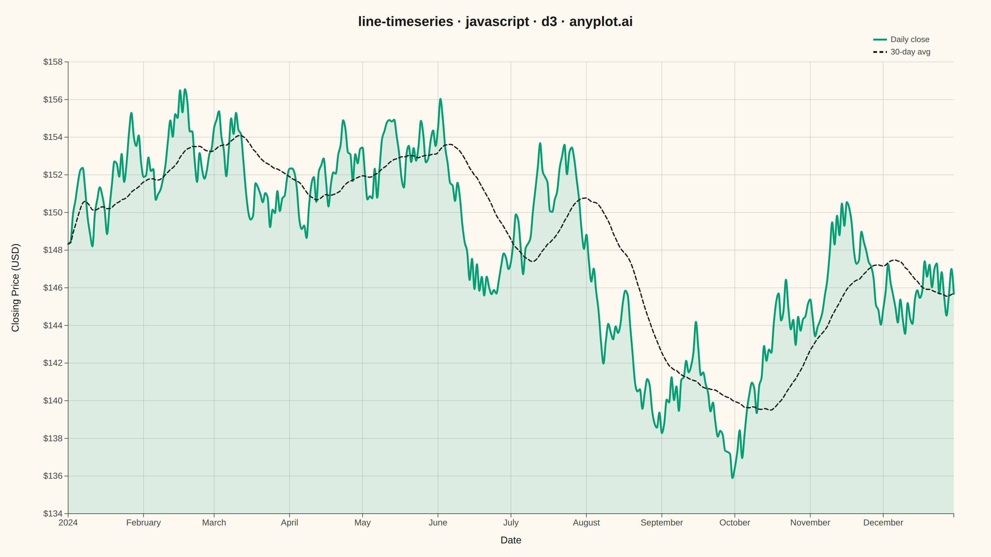
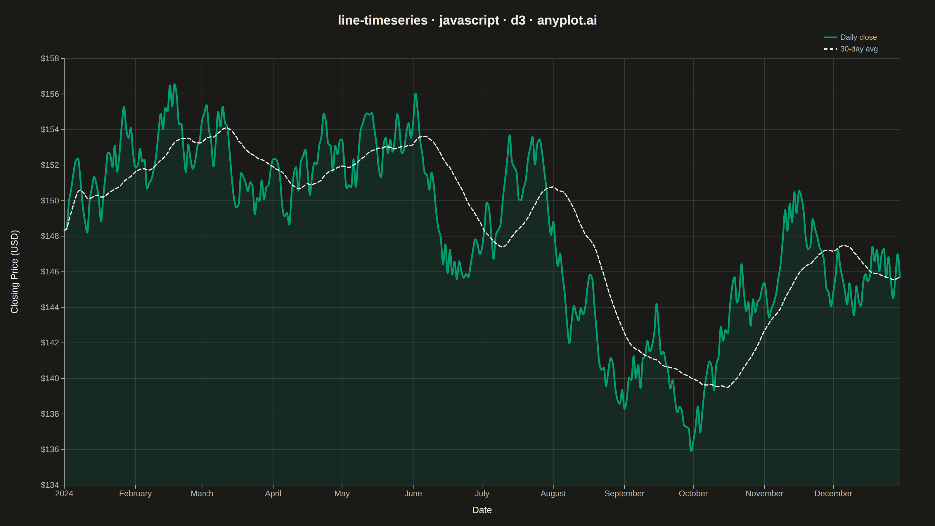
The same plot in 14 other libraries — JavaScript: Chart.js, Apache ECharts, Highcharts, MUI X Charts; Python: Altair, Bokeh, lets-plot, Matplotlib, Plotly, plotnine, Pygal, Seaborn; R: ggplot2; Julia: Makie.jl. Compare all 15 side by side: Time Series Line Plot in Python, R, Julia and JavaScript.
A time series line plot displays data points connected by lines over a datetime x-axis, with smart date formatting that automatically adjusts tick labels based on the time scale (days, months, years). This plot type is essential for temporal data analysis where proper date formatting and readability are critical. Unlike basic line plots, time series plots handle datetime parsing, timezone awareness, and intelligent tick label formatting.
// anyplot.ai
// line-timeseries: Time Series Line Plot
// Library: d3 7.9.0 | JavaScript 22.23.2
// Quality: 89/100 | Created: 2026-09-05

const t = window.ANYPLOT_TOKENS;
const { width, height } = window.ANYPLOT_SIZE;
const margin = { top: 100, right: 60, bottom: 70, left: 110 };
const iw = width - margin.left - margin.right;
const ih = height - margin.top - margin.bottom;

// --- Data: daily closing price random walk over one trading year -----------
function lcg(seed) {
  let state = seed;
  return () => {
    state = (state * 1103515245 + 12345) % 2147483648;
    return state / 2147483648;
  };
}
const random = lcg(42);

const startDate = new Date(2024, 0, 1);
let price = 148;
const data = Array.from({ length: 365 }, (_, i) => {
  const date = new Date(startDate);
  date.setDate(date.getDate() + i);
  price = Math.max(price + (random() - 0.485) * 3.4, 20);
  return { date, close: Math.round(price * 100) / 100 };
});

// --- 30-day rolling average via d3.cumsum prefix sums -----------------------
// Smooths the daily noise into a trend line, giving the viewer a focal point
// beyond the raw series (an expanding window for the first 29 days).
const WINDOW = 30;
const cum = d3.cumsum(data, (d) => d.close);
const rolling = data.map((d, i) => {
  const lo = Math.max(0, i - WINDOW + 1);
  const sum = cum[i] - (lo > 0 ? cum[lo - 1] : 0);
  return { date: d.date, avg: sum / (i - lo + 1) };
});

// --- Scales -------------------------------------------------------------
const x = d3.scaleTime().domain(d3.extent(data, (d) => d.date)).range([0, iw]);
const y = d3.scaleLinear().domain(d3.extent(data, (d) => d.close)).nice().range([ih, 0]);

// --- SVG mount ------------------------------------------------------------
const svg = d3.select("#container").append("svg").attr("width", width).attr("height", height);
const g = svg.append("g").attr("transform", `translate(${margin.left},${margin.top})`);

// --- Grid (drawn first, behind the line) ------------------------------------
const gridY = g.append("g").call(d3.axisLeft(y).tickSize(-iw).tickFormat(""));
gridY.selectAll("line").attr("stroke", t.grid);
gridY.select(".domain").remove();

const gridX = g
  .append("g")
  .attr("transform", `translate(0,${ih})`)
  .call(d3.axisBottom(x).ticks(10).tickSize(-ih).tickFormat(""));
gridX.selectAll("line").attr("stroke", t.grid);
gridX.select(".domain").remove();

// --- Area: subtle fill under the line to emphasize trend magnitude ---------
const area = d3
  .area()
  .x((d) => x(d.date))
  .y0(ih)
  .y1((d) => y(d.close))
  .curve(d3.curveMonotoneX);

g.append("path").datum(data).attr("fill", t.palette[0]).attr("fill-opacity", 0.12).attr("d", area);

// --- Line: intelligent date axis handles the temporal formatting -----------
const line = d3
  .line()
  .x((d) => x(d.date))
  .y((d) => y(d.close))
  .curve(d3.curveMonotoneX);

g.append("path")
  .datum(data)
  .attr("fill", "none")
  .attr("stroke", t.palette[0])
  .attr("stroke-width", 3)
  .attr("stroke-linejoin", "round")
  .attr("stroke-linecap", "round")
  .attr("d", line);

// --- Rolling average overlay: highlights the year's trend reversals ---------
const avgLine = d3
  .line()
  .x((d) => x(d.date))
  .y((d) => y(d.avg))
  .curve(d3.curveMonotoneX);

g.append("path")
  .datum(rolling)
  .attr("fill", "none")
  .attr("stroke", t.ink)
  .attr("stroke-width", 2)
  .attr("stroke-dasharray", "6,4")
  .attr("stroke-linecap", "round")
  .attr("d", avgLine);

// --- Axes -------------------------------------------------------------------
// d3's default time-scale tick format is already "smart": it switches
// resolution (year / month / day / hour) to match the ticks it selects for
// the current domain, so no custom multi-format function is needed here.
const xAxis = g.append("g").attr("transform", `translate(0,${ih})`).call(d3.axisBottom(x).ticks(10));
xAxis.selectAll("text").attr("fill", t.inkSoft).style("font-size", "14px");
xAxis.selectAll("line").attr("stroke", t.inkSoft);
xAxis.select(".domain").attr("stroke", t.inkSoft);

const yAxis = g.append("g").call(d3.axisLeft(y).tickFormat((d) => `$${d}`));
yAxis.selectAll("text").attr("fill", t.inkSoft).style("font-size", "14px");
yAxis.selectAll("line").attr("stroke", t.inkSoft);
yAxis.select(".domain").attr("stroke", t.inkSoft);

// --- Y-axis label -------------------------------------------------------
svg
  .append("text")
  .attr("transform", "rotate(-90)")
  .attr("x", -(margin.top + ih / 2))
  .attr("y", 30)
  .attr("text-anchor", "middle")
  .attr("fill", t.ink)
  .style("font-size", "16px")
  .text("Closing Price (USD)");

// --- X-axis label ---------------------------------------------------------
svg
  .append("text")
  .attr("x", margin.left + iw / 2)
  .attr("y", height - 22)
  .attr("text-anchor", "middle")
  .attr("fill", t.ink)
  .style("font-size", "16px")
  .text("Date");

// --- Title ------------------------------------------------------------------
svg
  .append("text")
  .attr("x", width / 2)
  .attr("y", 42)
  .attr("text-anchor", "middle")
  .attr("fill", t.ink)
  .style("font-size", "22px")
  .style("font-weight", "600")
  .text("line-timeseries · javascript · d3 · anyplot.ai");

// --- Legend: distinguishes the daily series from the smoothed trend --------
const legendItems = [
  { label: "Daily close", stroke: t.palette[0], dash: null },
  { label: "30-day avg", stroke: t.ink, dash: "6,4" },
];
const legendG = svg.append("g").attr("transform", `translate(${width - margin.right - 130},64)`);
legendItems.forEach((item, i) => {
  const row = legendG.append("g").attr("transform", `translate(0,${i * 20})`);
  row
    .append("line")
    .attr("x1", 0)
    .attr("x2", 22)
    .attr("y1", 0)
    .attr("y2", 0)
    .attr("stroke", item.stroke)
    .attr("stroke-width", 3)
    .attr("stroke-dasharray", item.dash);
  row.append("text").attr("x", 28).attr("y", 4).attr("fill", t.inkSoft).style("font-size", "13px").text(item.label);
});
Runnable source as JSON, for any HTTP client: https://api.anyplot.ai/specs/line-timeseries/d3/code. Any spec id and library id listed in llms-full.txt fit the same URL shape; every URL below is complete and callable.
{
  "spec_id": "line-timeseries",
  "language": "javascript",
  "library": "d3",
  "page": "https://anyplot.ai/line-timeseries/javascript/d3",
  "hub": "https://anyplot.ai/line-timeseries",
  "code_json": "https://api.anyplot.ai/specs/line-timeseries/d3/code",
  "spec_json": "https://api.anyplot.ai/specs/line-timeseries",
  "render_light_png": "https://storage.googleapis.com/anyplot-images/plots/line-timeseries/javascript/d3/plot-light.png",
  "render_dark_png": "https://storage.googleapis.com/anyplot-images/plots/line-timeseries/javascript/d3/plot-dark.png",
  "interactive_light_html": "https://storage.googleapis.com/anyplot-images/plots/line-timeseries/javascript/d3/plot-light.html",
  "interactive_dark_html": "https://storage.googleapis.com/anyplot-images/plots/line-timeseries/javascript/d3/plot-dark.html",
  "quality_score": 89.0,
  "license": "MIT",
  "guide": "https://anyplot.ai/llms.txt"
}
Part of Time Series Line Plot on anyplot.ai.