The same plot in 14 other libraries — Python: Altair, Bokeh, lets-plot, Matplotlib, Plotly, plotnine, Pygal, Seaborn; Julia: Makie.jl; JavaScript: Chart.js, D3.js, Apache ECharts, Highcharts, MUI X Charts. Compare all 15 side by side: Tile Grid Map for Equal-Area Geographic Comparison in Python, R, Julia and JavaScript.
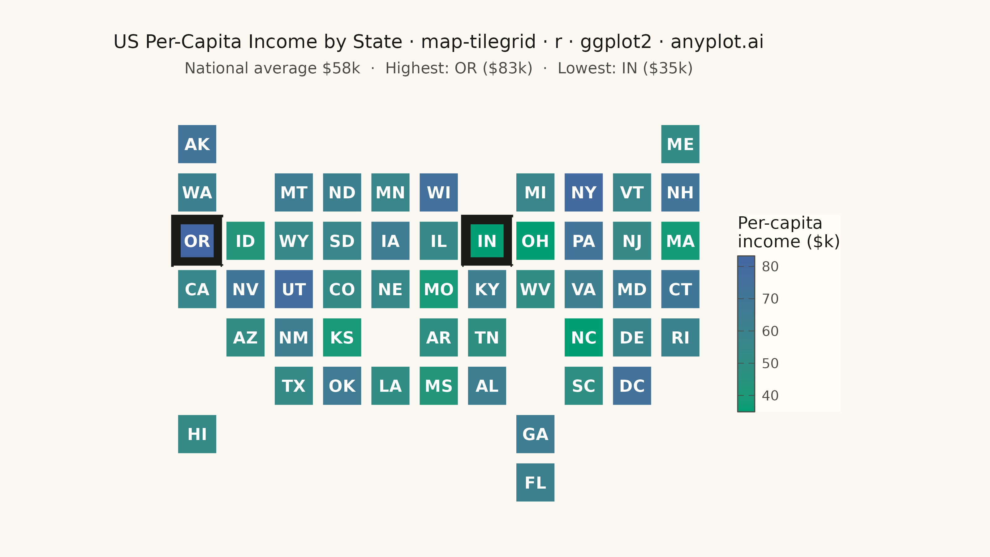
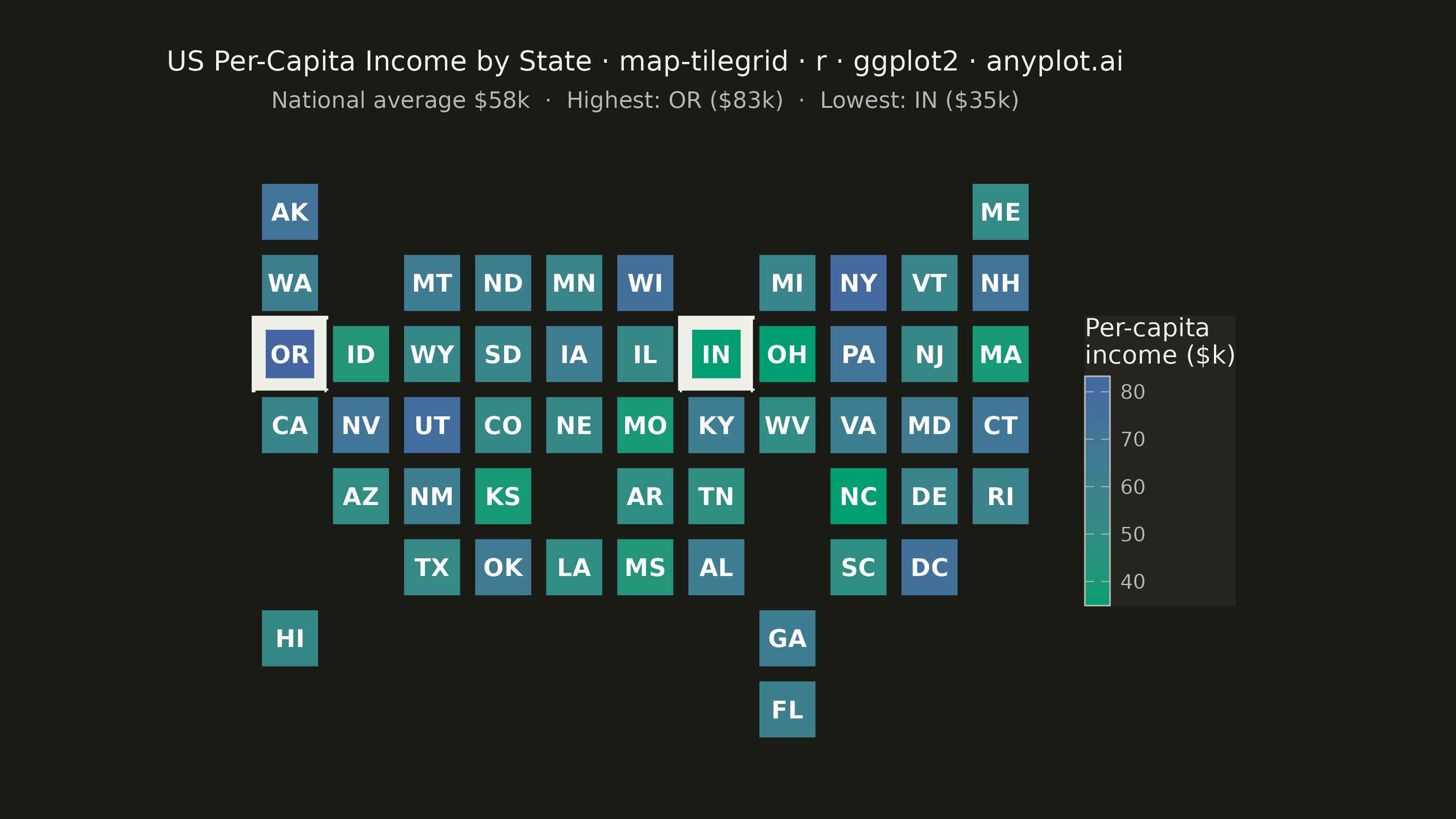
A tile grid map represents geographic regions (states, countries, provinces) as equally-sized tiles — squares or hexagons — arranged to approximate their real-world geographic positions. Unlike choropleth maps where large-area regions dominate visually, every region receives identical visual weight, making tile grid maps ideal for per-capita or per-region comparisons where the statistic matters more than physical area. Tiles are colored by a data variable and labeled with region abbreviations for identification.
#' anyplot.ai
#' map-tilegrid: Tile Grid Map for Equal-Area Geographic Comparison
#' Library: ggplot2 3.5.1 | R 4.4.1
#' Quality: 92/100 | Created: 2026-09-05

library(ggplot2)
library(dplyr)
library(ragg)

set.seed(42)

# --- Theme tokens (see prompts/default-style-guide.md "Theme-adaptive Chrome") ----
THEME       <- Sys.getenv("ANYPLOT_THEME", "light")
PAGE_BG     <- if (THEME == "light") "#FAF8F1" else "#1A1A17"
ELEVATED_BG <- if (THEME == "light") "#FFFDF6" else "#242420"
INK         <- if (THEME == "light") "#1A1A17" else "#F0EFE8"
INK_SOFT    <- if (THEME == "light") "#4A4A44" else "#B8B7B0"

# --- Data: US state tile grid + simulated per-capita income -----------------
# Row/col approximate each state's real-world position (0-indexed, top-left
# origin) so the tile layout still reads as a recognizable US map.
state_grid <- tibble::tribble(
  ~region, ~row, ~col,
  "AK", 0, 0,   "ME", 0, 10,
  "WA", 1, 0,   "MT", 1, 2,   "ND", 1, 3,   "MN", 1, 4,   "WI", 1, 5,
  "MI", 1, 7,   "NY", 1, 8,   "VT", 1, 9,   "NH", 1, 10,
  "OR", 2, 0,   "ID", 2, 1,   "WY", 2, 2,   "SD", 2, 3,   "IA", 2, 4,
  "IL", 2, 5,   "IN", 2, 6,   "OH", 2, 7,   "PA", 2, 8,   "NJ", 2, 9,
  "MA", 2, 10,
  "CA", 3, 0,   "NV", 3, 1,   "UT", 3, 2,   "CO", 3, 3,   "NE", 3, 4,
  "MO", 3, 5,   "KY", 3, 6,   "WV", 3, 7,   "VA", 3, 8,   "MD", 3, 9,
  "CT", 3, 10,
  "AZ", 4, 1,   "NM", 4, 2,   "KS", 4, 3,   "AR", 4, 5,   "TN", 4, 6,
  "NC", 4, 8,   "DE", 4, 9,   "RI", 4, 10,
  "TX", 5, 2,   "OK", 5, 3,   "LA", 5, 4,   "MS", 5, 5,   "AL", 5, 6,
  "SC", 5, 8,   "DC", 5, 9,
  "HI", 6, 0,   "GA", 6, 7,
  "FL", 7, 7
)

df <- state_grid %>%
  mutate(income_k = round(pmax(35, rnorm(n(), mean = 58, sd = 11)), 1))

# --- Outlier callouts (data-storytelling touch: national average + hi/lo) --
avg_income <- round(mean(df$income_k), 1)
top_state    <- dplyr::slice_max(df, income_k, n = 1, with_ties = FALSE)
bottom_state <- dplyr::slice_min(df, income_k, n = 1, with_ties = FALSE)

df <- df %>%
  mutate(
    is_outlier  = region %in% c(top_state$region, bottom_state$region),
    tile_color  = if_else(is_outlier, INK, PAGE_BG),   # neutral anchor for callout ring
    tile_stroke = if_else(is_outlier, 2.6, 1.2)
  )

# --- Title (fontsize scales with title length, see plot-generator.md) -------
title_text <- "US Per-Capita Income by State · map-tilegrid · r · ggplot2 · anyplot.ai"
title_n <- nchar(title_text, type = "chars")
title_size <- max(8, round(12 * min(1, 67 / title_n)))

subtitle_text <- sprintf(
  "National average $%.0fk  ·  Highest: %s ($%.0fk)  ·  Lowest: %s ($%.0fk)",
  avg_income, top_state$region, top_state$income_k,
  bottom_state$region, bottom_state$income_k
)

# --- Plot ---------------------------------------------------------------------
p <- ggplot(df, aes(x = col, y = -row)) +
  geom_tile(aes(fill = income_k, color = tile_color, linewidth = tile_stroke),
            width = 0.88, height = 0.88) +
  geom_text(aes(label = region), color = "#FFFFFF", size = 3.4,
            fontface = "bold") +
  scale_fill_gradient(low = "#009E73", high = "#4467A3",
                       name = "Per-capita\nincome ($k)",
                       guide = guide_colorbar(title.position = "top",
                                              barwidth  = grid::unit(0.35, "cm"),
                                              barheight = grid::unit(3.2, "cm"),
                                              frame.colour  = INK_SOFT,
                                              frame.linewidth = 0.3,
                                              ticks.colour  = INK_SOFT)) +
  scale_color_identity() +
  scale_linewidth_identity() +
  coord_fixed(ratio = 1, clip = "off") +
  labs(title = title_text, subtitle = subtitle_text) +
  theme_void(base_size = 8) +
  theme(
    plot.background    = element_rect(fill = PAGE_BG, color = PAGE_BG),
    panel.background   = element_rect(fill = PAGE_BG, color = NA),
    plot.title          = element_text(color = INK, size = title_size,
                                        hjust = 0.5,
                                        margin = margin(b = 6)),
    plot.subtitle       = element_text(color = INK_SOFT, size = 9,
                                        hjust = 0.5,
                                        margin = margin(b = 16)),
    legend.position     = "right",
    legend.background   = element_rect(fill = ELEVATED_BG, color = NA),
    legend.title        = element_text(color = INK, size = 10),
    legend.text         = element_text(color = INK_SOFT, size = 8),
    legend.key.height   = grid::unit(1.1, "cm"),
    plot.margin         = margin(t = 20, r = 30, b = 20, l = 30)
  )

# --- Save (both themes, ragg device, see prompts/library/ggplot2.md) --------
ggsave(
  filename = sprintf("plot-%s.png", THEME),
  plot     = p,
  device   = ragg::agg_png,
  width    = 8,
  height   = 4.5,
  units    = "in",
  dpi      = 400
)
Runnable source as JSON, for any HTTP client: https://api.anyplot.ai/specs/map-tilegrid/ggplot2/code. Any spec id and library id listed in llms-full.txt fit the same URL shape; every URL below is complete and callable.
{
  "spec_id": "map-tilegrid",
  "language": "r",
  "library": "ggplot2",
  "page": "https://anyplot.ai/map-tilegrid/r/ggplot2",
  "hub": "https://anyplot.ai/map-tilegrid",
  "code_json": "https://api.anyplot.ai/specs/map-tilegrid/ggplot2/code",
  "spec_json": "https://api.anyplot.ai/specs/map-tilegrid",
  "render_light_png": "https://storage.googleapis.com/anyplot-images/plots/map-tilegrid/r/ggplot2/plot-light.png",
  "render_dark_png": "https://storage.googleapis.com/anyplot-images/plots/map-tilegrid/r/ggplot2/plot-dark.png",
  "quality_score": 92.0,
  "license": "MIT",
  "guide": "https://anyplot.ai/llms.txt"
}
Part of Tile Grid Map for Equal-Area Geographic Comparison on anyplot.ai.