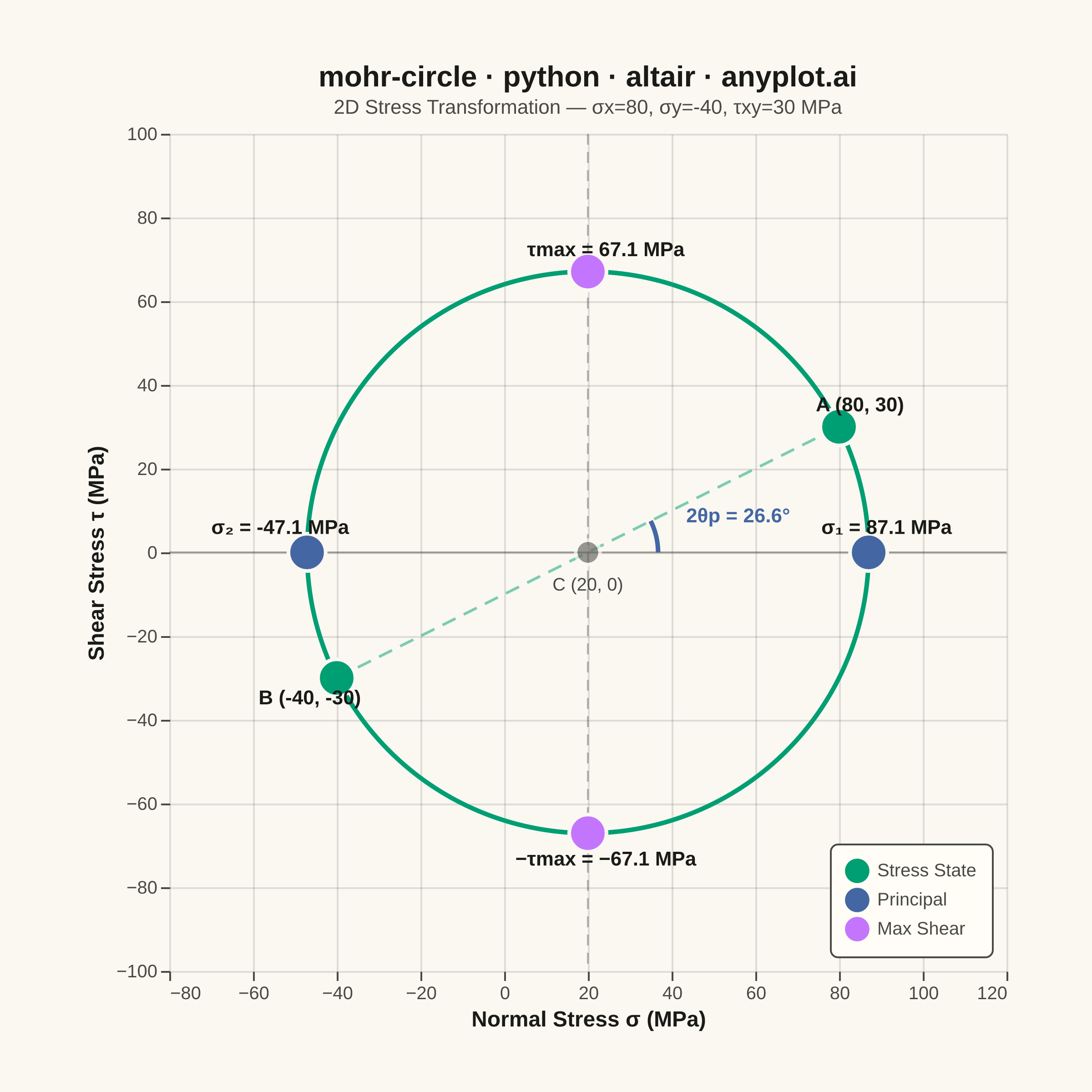
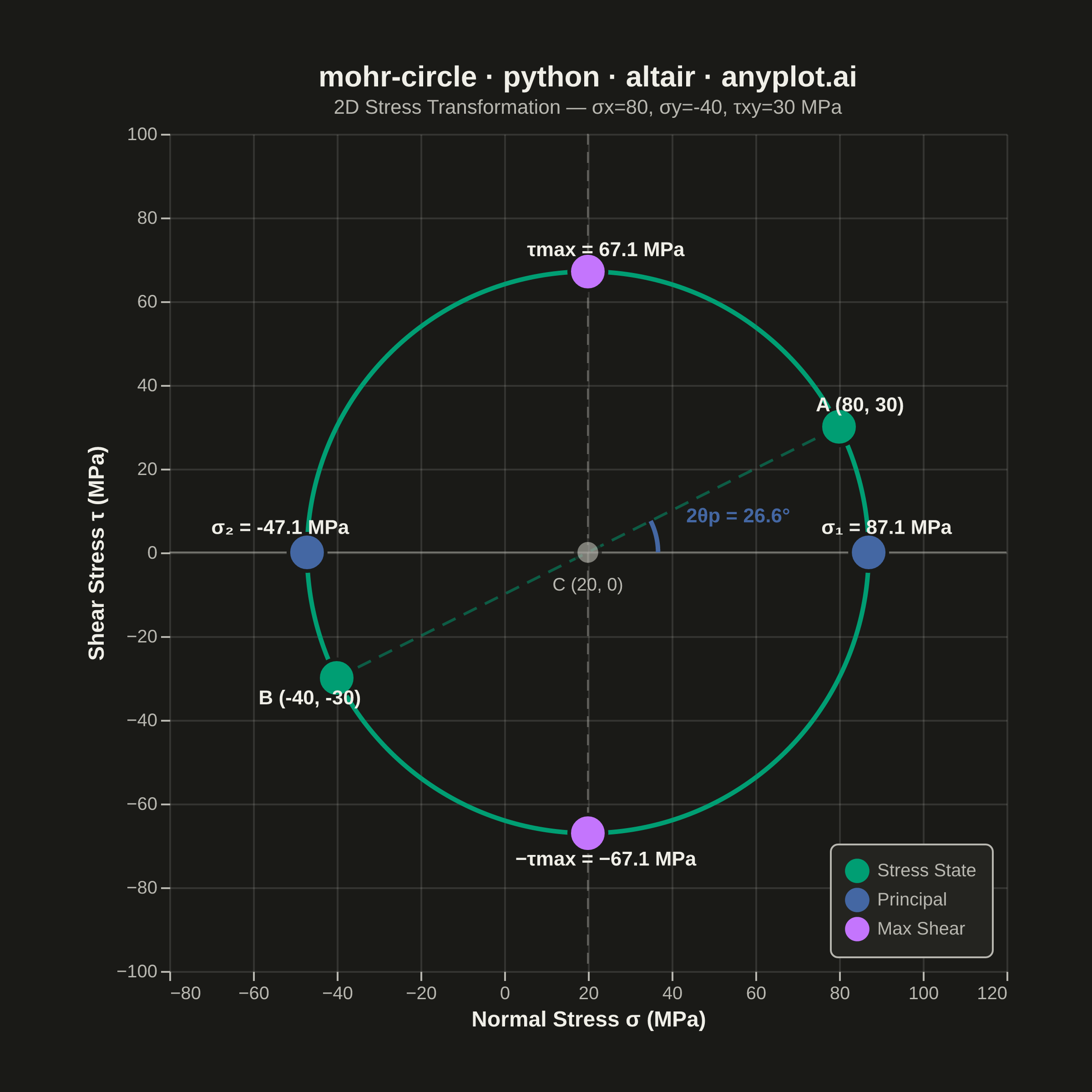
Mohr's Circle is a graphical method used to determine principal stresses, maximum shear stress, and stress transformations from a given 2D stress state. A circle is drawn on a normal stress (σ) vs. shear stress (τ) plane, with the center at ((σx + σy) / 2, 0) and a radius derived from the stress components. It is an essential tool in mechanical and civil engineering for visualizing how stress components change under coordinate rotation.
""" anyplot.ai
mohr-circle: Mohr's Circle for Stress Analysis
Library: altair 6.1.0 | Python 3.13.13
Quality: 91/100 | Updated: 2026-05-30
"""

import os
import sys


# altair.py shadows the altair package — remove this directory from sys.path first
_here = os.path.dirname(os.path.abspath(__file__))
sys.path[:] = [p for p in sys.path if os.path.realpath(p or os.getcwd()) != os.path.realpath(_here)]

import altair as alt
import numpy as np
import pandas as pd
from PIL import Image


# Theme tokens (Imprint style guide)
THEME = os.getenv("ANYPLOT_THEME", "light")
PAGE_BG = "#FAF8F1" if THEME == "light" else "#1A1A17"
ELEVATED_BG = "#FFFDF6" if THEME == "light" else "#242420"
INK = "#1A1A17" if THEME == "light" else "#F0EFE8"
INK_SOFT = "#4A4A44" if THEME == "light" else "#B8B7B0"
INK_MUTED = "#6B6A63" if THEME == "light" else "#A8A79F"

# Imprint palette positions used
BRAND = "#009E73"  # pos 1 — stress state points + circle line
LAVENDER = "#C475FD"  # pos 2 — max shear points
BLUE = "#4467A3"  # pos 3 — principal stresses + 2θp arc

# Data — 2D stress state (MPa)
sigma_x = 80
sigma_y = -40
tau_xy = 30

center = (sigma_x + sigma_y) / 2
radius = np.sqrt(((sigma_x - sigma_y) / 2) ** 2 + tau_xy**2)
sigma_1 = center + radius
sigma_2 = center - radius
tau_max = radius
theta_p2 = np.degrees(np.arctan2(tau_xy, (sigma_x - sigma_y) / 2))

# Circle outline (parametric)
angles = np.linspace(0, 2 * np.pi, 361)
circle_df = pd.DataFrame(
    {"sigma": center + radius * np.cos(angles), "tau": radius * np.sin(angles), "order": range(361)}
)

# Key stress points
stress_points = pd.DataFrame(
    [
        {
            "sigma": sigma_x,
            "tau": tau_xy,
            "label": f"A ({sigma_x}, {tau_xy})",
            "type": "Stress State",
            "dx": 14,
            "dy": -14,
        },
        {
            "sigma": sigma_y,
            "tau": -tau_xy,
            "label": f"B ({sigma_y}, {-tau_xy})",
            "type": "Stress State",
            "dx": -18,
            "dy": 14,
        },
        {"sigma": sigma_1, "tau": 0, "label": f"σ₁ = {sigma_1:.1f} MPa", "type": "Principal", "dx": 12, "dy": -16},
        {"sigma": sigma_2, "tau": 0, "label": f"σ₂ = {sigma_2:.1f} MPa", "type": "Principal", "dx": -18, "dy": -16},
        {
            "sigma": center,
            "tau": tau_max,
            "label": f"τmax = {tau_max:.1f} MPa",
            "type": "Max Shear",
            "dx": 12,
            "dy": -14,
        },
        {
            "sigma": center,
            "tau": -tau_max,
            "label": f"−τmax = −{tau_max:.1f} MPa",
            "type": "Max Shear",
            "dx": 12,
            "dy": 18,
        },
    ]
)

# Diameter line A → B
diameter_df = pd.DataFrame({"sigma": [sigma_x, sigma_y], "tau": [tau_xy, -tau_xy]})

# 2θp angle arc
arc_r = radius * 0.25
arc_angles = np.linspace(0, np.radians(theta_p2), 50)
arc_df = pd.DataFrame(
    {"sigma": center + arc_r * np.cos(arc_angles), "tau": arc_r * np.sin(arc_angles), "order": range(50)}
)

# Equal-aspect domains — square inner view (460×460) so circle renders as true circle
span = max(sigma_1 - sigma_2, 2 * tau_max) + 30
domain_sigma = [center - span / 2, center + span / 2]
domain_tau = [-span / 2, span / 2]

x_scale = alt.Scale(domain=domain_sigma)
y_scale = alt.Scale(domain=domain_tau)

# Reference lines through center
h_rule = (
    alt.Chart(pd.DataFrame({"tau": [0]}))
    .mark_rule(color=INK_SOFT, strokeWidth=1, opacity=0.5)
    .encode(y=alt.Y("tau:Q", scale=y_scale))
)
v_rule = (
    alt.Chart(pd.DataFrame({"sigma": [center]}))
    .mark_rule(color=INK_SOFT, strokeWidth=1, opacity=0.4, strokeDash=[6, 4])
    .encode(x=alt.X("sigma:Q", scale=x_scale))
)

# Circle
circle = (
    alt.Chart(circle_df)
    .mark_line(color=BRAND, strokeWidth=2.5)
    .encode(
        x=alt.X("sigma:Q", title="Normal Stress σ (MPa)", scale=x_scale),
        y=alt.Y("tau:Q", title="Shear Stress τ (MPa)", scale=y_scale),
        order="order:Q",
    )
)

# Diameter line
diameter = (
    alt.Chart(diameter_df)
    .mark_line(color=BRAND, strokeWidth=1.5, strokeDash=[8, 5], opacity=0.5)
    .encode(x="sigma:Q", y="tau:Q")
)

# 2θp arc — linked to principal plane rotation
arc = alt.Chart(arc_df).mark_line(color=BLUE, strokeWidth=2.5).encode(x="sigma:Q", y="tau:Q", order="order:Q")

# Angle label
angle_lbl_df = pd.DataFrame(
    {
        "sigma": [center + arc_r * 2.2 * np.cos(np.radians(theta_p2 / 2))],
        "tau": [arc_r * 2.2 * np.sin(np.radians(theta_p2 / 2))],
    }
)
angle_lbl = (
    alt.Chart(angle_lbl_df)
    .mark_text(text=f"2θp = {theta_p2:.1f}°", fontSize=11, fontWeight="bold", color=BLUE)
    .encode(x="sigma:Q", y="tau:Q")
)

# Interactive hover selection (enhances HTML output)
highlight = alt.selection_point(fields=["type"], on="pointerover")

# Stress points with Imprint palette colors and hover interaction
points = (
    alt.Chart(stress_points)
    .mark_point(filled=True, strokeWidth=2, stroke=PAGE_BG)
    .encode(
        x="sigma:Q",
        y="tau:Q",
        color=alt.Color(
            "type:N",
            scale=alt.Scale(domain=["Stress State", "Principal", "Max Shear"], range=[BRAND, BLUE, LAVENDER]),
            legend=alt.Legend(
                title=None,
                orient="bottom-right",
                direction="vertical",
                symbolSize=180,
                symbolStrokeWidth=0,
                labelFontSize=10,
                padding=8,
                offset=8,
                cornerRadius=4,
            ),
        ),
        size=alt.condition(highlight, alt.value(420), alt.value(300)),
        opacity=alt.condition(highlight, alt.value(1.0), alt.value(0.85)),
        tooltip=[
            alt.Tooltip("label:N", title="Point"),
            alt.Tooltip("sigma:Q", title="σ (MPa)", format=".1f"),
            alt.Tooltip("tau:Q", title="τ (MPa)", format=".1f"),
            alt.Tooltip("type:N", title="Category"),
        ],
    )
    .add_params(highlight)
)

# Center point
center_pt_df = pd.DataFrame({"sigma": [center], "tau": [0]})
center_pt = (
    alt.Chart(center_pt_df)
    .mark_point(size=180, filled=True, color=INK_MUTED, strokeWidth=2, stroke=PAGE_BG)
    .encode(x="sigma:Q", y="tau:Q")
)
center_lbl = (
    alt.Chart(center_pt_df)
    .mark_text(text=f"C ({center:.0f}, 0)", fontSize=10, color=INK_SOFT, dy=18)
    .encode(x="sigma:Q", y="tau:Q")
)

# Annotation labels — data-space offsets (px_to_data = span per inner-view pixel)
px_to_data = span / 460
stress_points["lbl_sigma"] = stress_points["sigma"] + stress_points["dx"] * px_to_data
stress_points["lbl_tau"] = stress_points["tau"] - stress_points["dy"] * px_to_data
labels = (
    alt.Chart(stress_points)
    .mark_text(fontSize=11, fontWeight="bold", color=INK)
    .encode(x="lbl_sigma:Q", y="lbl_tau:Q", text="label:N")
)

# Title and subtitle
title_text = "mohr-circle · python · altair · anyplot.ai"
subtitle_text = f"2D Stress Transformation — σx={sigma_x}, σy={sigma_y}, τxy={tau_xy} MPa"

# Compose chart — square inner view (460×460) preserves circular aspect ratio
chart = (
    alt.layer(h_rule, v_rule, circle, diameter, arc, points, center_pt, labels, center_lbl, angle_lbl)
    .properties(
        width=460,
        height=460,
        background=PAGE_BG,
        title=alt.Title(
            title_text,
            fontSize=16,
            fontWeight="bold",
            color=INK,
            subtitle=subtitle_text,
            subtitleFontSize=11,
            subtitleColor=INK_SOFT,
        ),
    )
    .configure_view(fill=PAGE_BG, strokeWidth=0, continuousWidth=460, continuousHeight=460)
    .configure_axis(
        labelFontSize=10,
        titleFontSize=12,
        titleColor=INK,
        labelColor=INK_SOFT,
        tickColor=INK_SOFT,
        grid=True,
        gridOpacity=0.12,
        gridColor=INK,
        domain=False,
    )
    .configure_legend(
        fillColor=ELEVATED_BG,
        strokeColor=INK_SOFT,
        labelColor=INK_SOFT,
        titleColor=INK,
        labelFontSize=10,
        titleFontSize=10,
    )
    .configure_title(color=INK)
)

# Save — target 2400×2400; pad with PAGE_BG if vl-convert lands short
TW, TH = 2400, 2400
chart.save(f"plot-{THEME}.png", scale_factor=4.0)

_img = Image.open(f"plot-{THEME}.png").convert("RGB")
_w, _h = _img.size
if _w > TW or _h > TH:
    raise SystemExit(
        f"altair vl-convert produced {_w}×{_h}, exceeds target {TW}×{TH}. "
        f"Shrink chart .properties(width=, height=) values and re-render."
    )
if _w < TW or _h < TH:
    _canvas = Image.new("RGB", (TW, TH), PAGE_BG)
    _canvas.paste(_img, ((TW - _w) // 2, (TH - _h) // 2))
    _canvas.save(f"plot-{THEME}.png")

chart.save(f"plot-{THEME}.html")
Runnable source as JSON, for any HTTP client: https://api.anyplot.ai/specs/mohr-circle/altair/code. Any spec id and library id listed in llms-full.txt fit the same URL shape; every URL below is complete and callable.
{
  "spec_id": "mohr-circle",
  "language": "python",
  "library": "altair",
  "page": "https://anyplot.ai/mohr-circle/python/altair",
  "hub": "https://anyplot.ai/mohr-circle",
  "code_json": "https://api.anyplot.ai/specs/mohr-circle/altair/code",
  "spec_json": "https://api.anyplot.ai/specs/mohr-circle",
  "render_light_png": "https://storage.googleapis.com/anyplot-images/plots/mohr-circle/python/altair/plot-light.png",
  "render_dark_png": "https://storage.googleapis.com/anyplot-images/plots/mohr-circle/python/altair/plot-dark.png",
  "interactive_light_html": "https://storage.googleapis.com/anyplot-images/plots/mohr-circle/python/altair/plot-light.html",
  "interactive_dark_html": "https://storage.googleapis.com/anyplot-images/plots/mohr-circle/python/altair/plot-dark.html",
  "quality_score": 91.0,
  "license": "MIT",
  "guide": "https://anyplot.ai/llms.txt"
}
Part of Mohr's Circle for Stress Analysis on anyplot.ai.