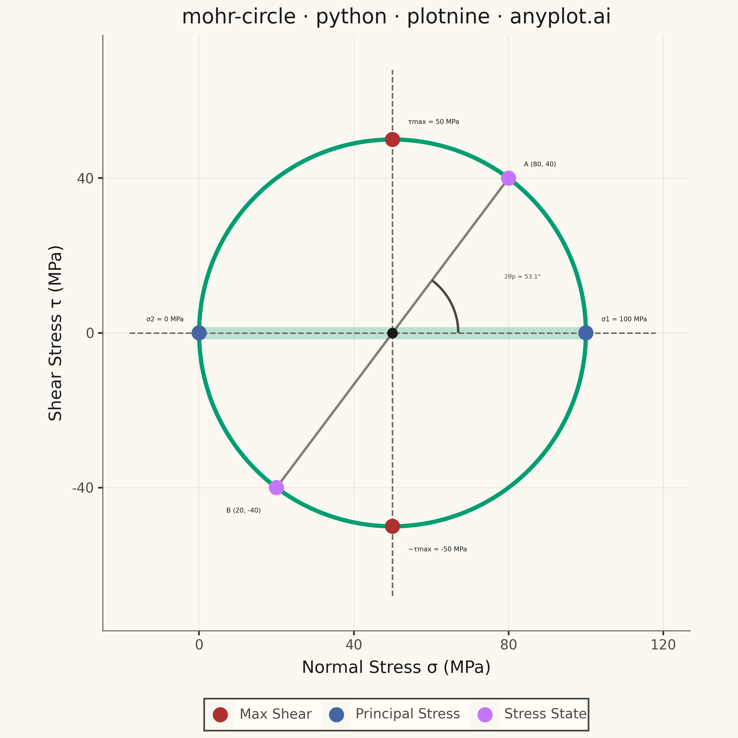
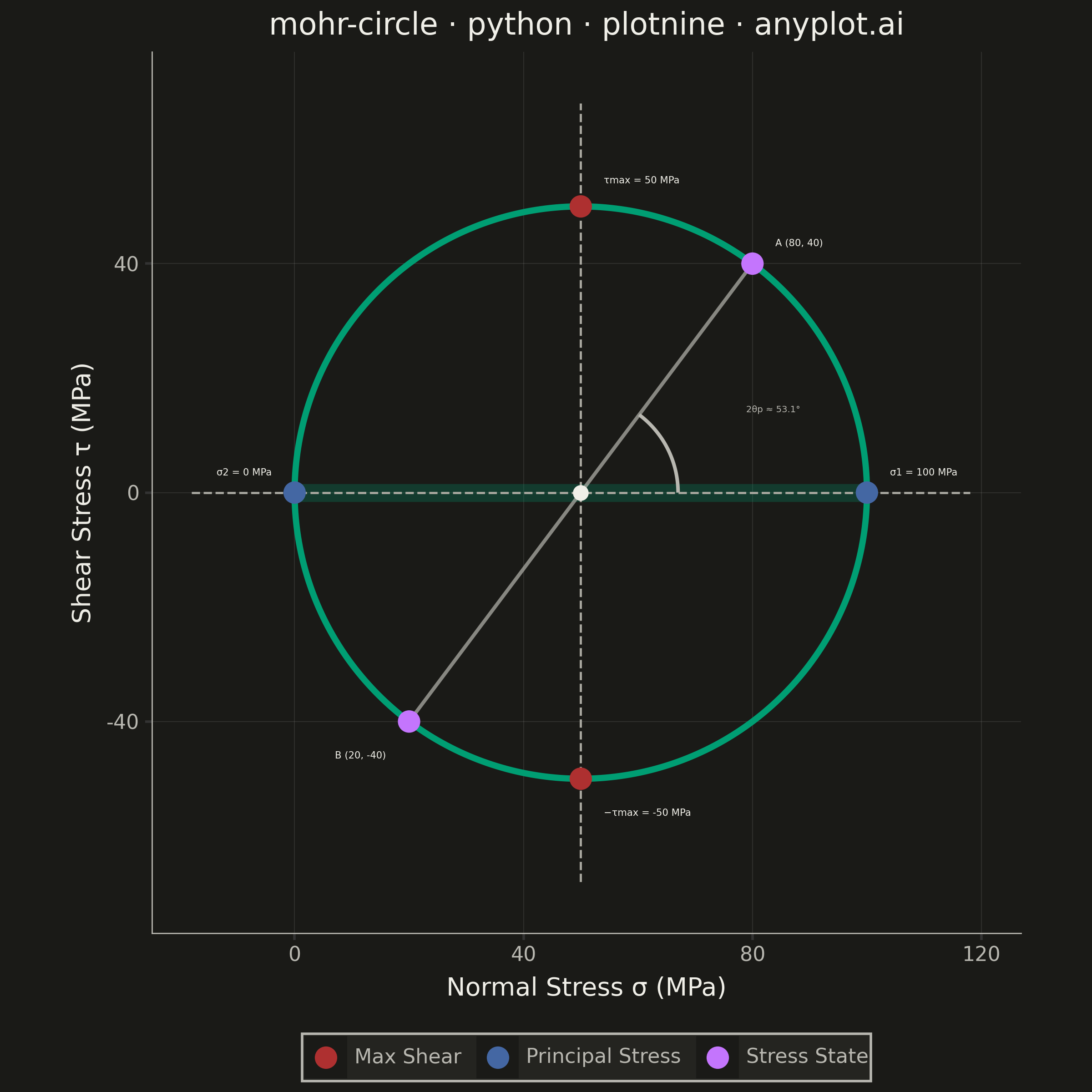
The same plot in 14 other libraries — Python: Altair, Bokeh, lets-plot, Matplotlib, Plotly, Pygal, Seaborn; R: ggplot2; Julia: Makie.jl; JavaScript: Chart.js, D3.js, Apache ECharts, Highcharts, MUI X Charts. Compare all 15 side by side: Mohr's Circle for Stress Analysis in Python, R, Julia and JavaScript.
Mohr's Circle is a graphical method used to determine principal stresses, maximum shear stress, and stress transformations from a given 2D stress state. A circle is drawn on a normal stress (σ) vs. shear stress (τ) plane, with the center at ((σx + σy) / 2, 0) and a radius derived from the stress components. It is an essential tool in mechanical and civil engineering for visualizing how stress components change under coordinate rotation.
""" anyplot.ai
mohr-circle: Mohr's Circle for Stress Analysis
Library: plotnine 0.15.4 | Python 3.13.13
Quality: 88/100 | Created: 2026-05-30
"""

import os
import sys

import numpy as np
import pandas as pd


# Work around naming conflict: plotnine.py vs plotnine package
script_dir = os.path.dirname(os.path.abspath(__file__))
for _p in (script_dir, "", "."):
    if _p in sys.path:
        sys.path.remove(_p)

from plotnine import (
    aes,
    coord_fixed,
    element_blank,
    element_line,
    element_rect,
    element_text,
    geom_path,
    geom_point,
    geom_segment,
    geom_text,
    ggplot,
    labs,
    scale_color_manual,
    theme,
)


# Theme tokens — Imprint palette
THEME = os.getenv("ANYPLOT_THEME", "light")
PAGE_BG = "#FAF8F1" if THEME == "light" else "#1A1A17"
ELEVATED_BG = "#FFFDF6" if THEME == "light" else "#242420"
INK = "#1A1A17" if THEME == "light" else "#F0EFE8"
INK_SOFT = "#4A4A44" if THEME == "light" else "#B8B7B0"
INK_MUTED = "#6B6A63" if THEME == "light" else "#A8A79F"

IMPRINT_PALETTE = ["#009E73", "#C475FD", "#4467A3", "#BD8233", "#AE3030", "#2ABCCD", "#954477", "#99B314"]
BRAND = IMPRINT_PALETTE[0]  # Mohr's circle — always first categorical series

# Stress state: steel shaft under bending + torsion (MPa)
sigma_x = 80.0
sigma_y = 20.0
tau_xy = 40.0

# Derived stress quantities
sigma_c = (sigma_x + sigma_y) / 2
radius = np.sqrt(((sigma_x - sigma_y) / 2) ** 2 + tau_xy**2)
sigma_1 = sigma_c + radius
sigma_2 = sigma_c - radius
tau_max = radius
two_theta_p = np.degrees(np.arctan2(tau_xy, (sigma_x - sigma_y) / 2))

# Mohr's circle path
angles = np.linspace(0, 2 * np.pi, 361)
circle_df = pd.DataFrame({"sigma": sigma_c + radius * np.cos(angles), "tau": radius * np.sin(angles)})

# Angle arc from σ-axis to line CA (visualising 2θp)
angle_A = np.arctan2(tau_xy, sigma_x - sigma_c)
arc_r = radius * 0.34
arc_df = pd.DataFrame(
    {"sigma": sigma_c + arc_r * np.cos(np.linspace(0, angle_A, 60)), "tau": arc_r * np.sin(np.linspace(0, angle_A, 60))}
)

# Reference lines: horizontal σ-axis and vertical through center
pad = 18.0
ref_df = pd.DataFrame(
    {
        "x": [sigma_2 - pad, sigma_c],
        "xend": [sigma_1 + pad, sigma_c],
        "y": [0.0, -tau_max - pad],
        "yend": [0.0, tau_max + pad],
    }
)

# Diameter from A(σx, τxy) to B(σy, −τxy)
diam_df = pd.DataFrame({"x": [sigma_x], "xend": [sigma_y], "y": [tau_xy], "yend": [-tau_xy]})

# Key points with engineering roles
points_df = pd.DataFrame(
    {
        "sigma": [sigma_x, sigma_y, sigma_1, sigma_2, sigma_c, sigma_c],
        "tau": [tau_xy, -tau_xy, 0.0, 0.0, tau_max, -tau_max],
        "role": ["Stress State", "Stress State", "Principal Stress", "Principal Stress", "Max Shear", "Max Shear"],
    }
)

center_df = pd.DataFrame({"sigma": [sigma_c], "tau": [0.0]})

# Accent segment along x-axis between σ2 and σ1 — draws eye to the principal stress result
span_df = pd.DataFrame({"x": [sigma_2], "xend": [sigma_1], "y": [0.0], "yend": [0.0]})

# 2θp arc label — bisecting angle, outside the arc
angle_mid = angle_A / 2
arc_lbl_df = pd.DataFrame(
    {
        "sigma": [sigma_c + arc_r * 1.9 * np.cos(angle_mid)],
        "tau": [arc_r * 1.9 * np.sin(angle_mid)],
        "label": [f"2θp ≈ {two_theta_p:.1f}°"],
    }
)

# Labels left-aligned (text extends rightward from anchor)
labels_left = pd.DataFrame(
    {
        "sigma": [sigma_x + 4.0, sigma_1 + 4.0, sigma_c + 4.0, sigma_c + 4.0],
        "tau": [tau_xy + 3.5, 3.5, tau_max + 4.5, -tau_max - 6.0],
        "label": [
            f"A ({sigma_x:.0f}, {tau_xy:.0f})",
            f"σ1 = {sigma_1:.0f} MPa",
            f"τmax = {tau_max:.0f} MPa",
            f"−τmax = {-tau_max:.0f} MPa",
        ],
    }
)

# Labels right-aligned (text extends leftward from anchor)
labels_right = pd.DataFrame(
    {
        "sigma": [sigma_y - 4.0, sigma_2 - 4.0],
        "tau": [-tau_xy - 6.0, 3.5],
        "label": [f"B ({sigma_y:.0f}, {-tau_xy:.0f})", f"σ2 = {sigma_2:.0f} MPa"],
    }
)

title = "mohr-circle · python · plotnine · anyplot.ai"

anyplot_theme = theme(
    figure_size=(6, 6),
    plot_background=element_rect(fill=PAGE_BG, color=PAGE_BG),
    panel_background=element_rect(fill=PAGE_BG),
    panel_grid_major=element_line(color=INK, size=0.3, alpha=0.12),
    panel_grid_minor=element_blank(),
    panel_border=element_blank(),
    axis_title=element_text(color=INK, size=10),
    axis_text=element_text(color=INK_SOFT, size=8),
    axis_line=element_line(color=INK_SOFT, size=0.5),
    plot_title=element_text(color=INK, size=12, ha="center"),
    legend_background=element_rect(fill=ELEVATED_BG, color=INK_SOFT),
    legend_text=element_text(color=INK_SOFT, size=8),
    legend_title=element_blank(),
    legend_position="bottom",
)

plot = (
    ggplot(circle_df, aes(x="sigma", y="tau"))
    # Accent segment from σ2 to σ1 — guides eye to the principal stress result
    + geom_segment(data=span_df, mapping=aes(x="x", xend="xend", y="y", yend="yend"), color=BRAND, size=4.0, alpha=0.25)
    # Dashed reference lines through center
    + geom_segment(
        data=ref_df, mapping=aes(x="x", xend="xend", y="y", yend="yend"), color=INK_MUTED, size=0.5, linetype="dashed"
    )
    # Diameter line from A to B
    + geom_segment(
        data=diam_df, mapping=aes(x="x", xend="xend", y="y", yend="yend"), color=INK_SOFT, size=0.8, alpha=0.7
    )
    # Mohr's circle — Imprint position 1 (brand green)
    + geom_path(color=BRAND, size=1.4)
    # Angle arc annotating 2θp
    + geom_path(data=arc_df, color=INK_SOFT, size=0.8)
    # Key points colored by engineering role
    + geom_point(data=points_df, mapping=aes(color="role"), size=4.0)
    + scale_color_manual(
        values={
            "Stress State": IMPRINT_PALETTE[1],
            "Principal Stress": IMPRINT_PALETTE[2],
            "Max Shear": IMPRINT_PALETTE[4],
        },
        name="",
    )
    # Center mark C
    + geom_point(data=center_df, color=INK, size=2.5)
    # Left-aligned labels
    + geom_text(data=labels_left, mapping=aes(label="label"), ha="left", size=3.8, color=INK)
    # Right-aligned labels
    + geom_text(data=labels_right, mapping=aes(label="label"), ha="right", size=3.8, color=INK)
    # Angle arc label
    + geom_text(data=arc_lbl_df, mapping=aes(label="label"), ha="left", size=3.5, color=INK_SOFT)
    + labs(x="Normal Stress σ (MPa)", y="Shear Stress τ (MPa)", title=title)
    + coord_fixed(ratio=1, xlim=(-18, 120), ylim=(-70, 70))
    + anyplot_theme
)

plot.save(f"plot-{THEME}.png", dpi=400, width=6, height=6, units="in")
Runnable source as JSON, for any HTTP client: https://api.anyplot.ai/specs/mohr-circle/plotnine/code. Any spec id and library id listed in llms-full.txt fit the same URL shape; every URL below is complete and callable.
{
  "spec_id": "mohr-circle",
  "language": "python",
  "library": "plotnine",
  "page": "https://anyplot.ai/mohr-circle/python/plotnine",
  "hub": "https://anyplot.ai/mohr-circle",
  "code_json": "https://api.anyplot.ai/specs/mohr-circle/plotnine/code",
  "spec_json": "https://api.anyplot.ai/specs/mohr-circle",
  "render_light_png": "https://storage.googleapis.com/anyplot-images/plots/mohr-circle/python/plotnine/plot-light.png",
  "render_dark_png": "https://storage.googleapis.com/anyplot-images/plots/mohr-circle/python/plotnine/plot-dark.png",
  "quality_score": 88.0,
  "license": "MIT",
  "guide": "https://anyplot.ai/llms.txt"
}
Part of Mohr's Circle for Stress Analysis on anyplot.ai.