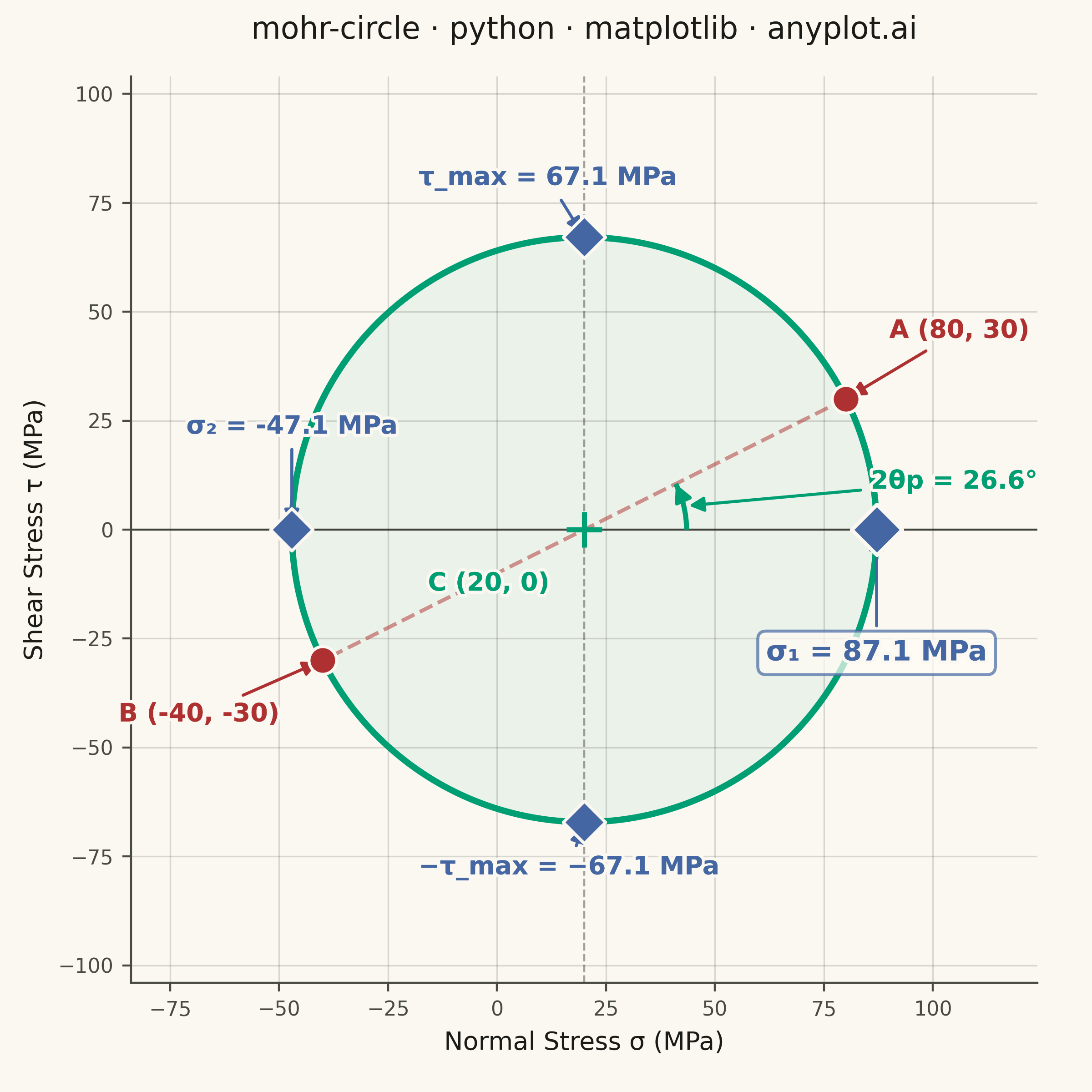
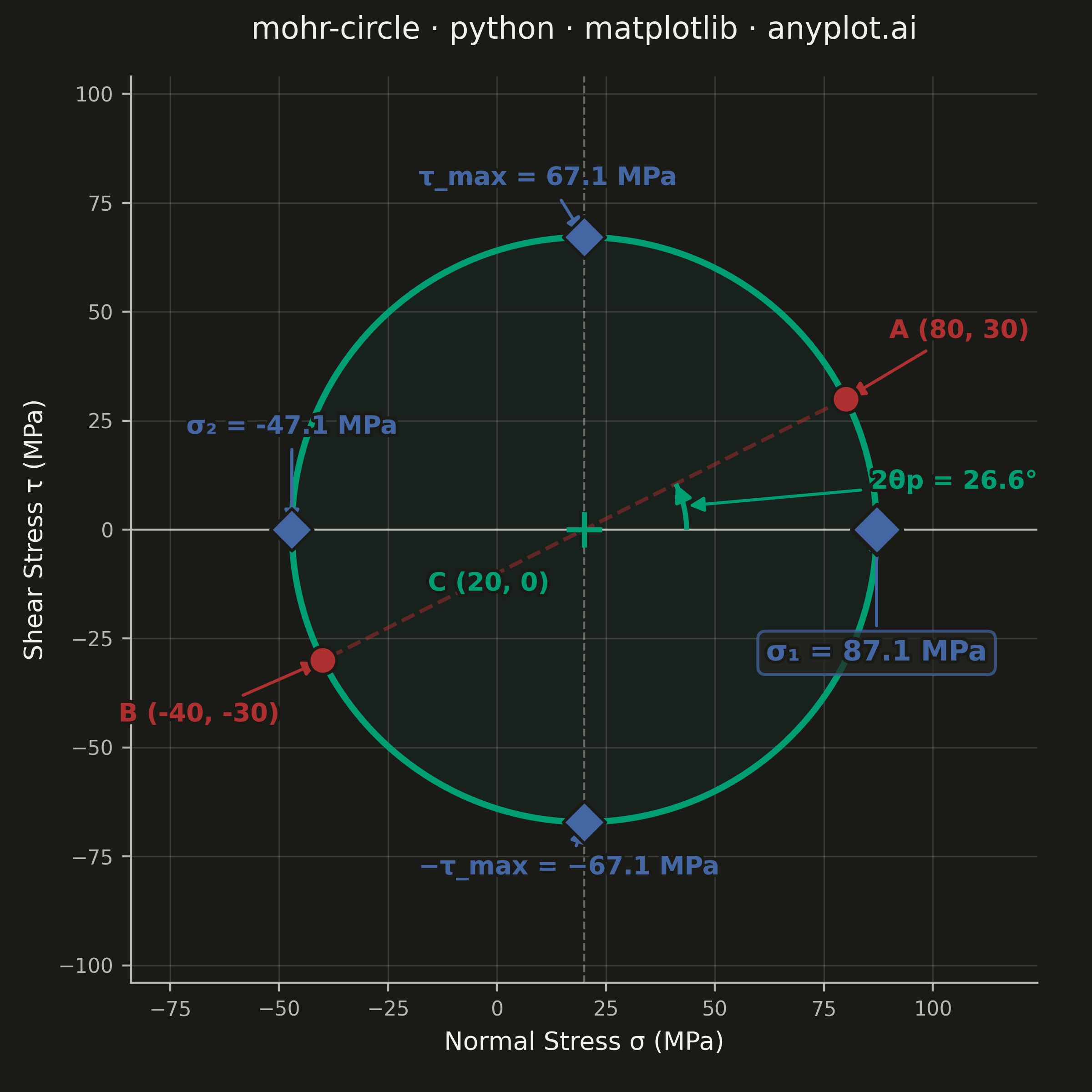
Mohr's Circle is a graphical method used to determine principal stresses, maximum shear stress, and stress transformations from a given 2D stress state. A circle is drawn on a normal stress (σ) vs. shear stress (τ) plane, with the center at ((σx + σy) / 2, 0) and a radius derived from the stress components. It is an essential tool in mechanical and civil engineering for visualizing how stress components change under coordinate rotation.
""" anyplot.ai
mohr-circle: Mohr's Circle for Stress Analysis
Library: matplotlib 3.10.9 | Python 3.13.13
Quality: 87/100 | Updated: 2026-05-30
"""

import os

import matplotlib.patches as patches
import matplotlib.patheffects as patheffects
import matplotlib.pyplot as plt
import numpy as np


# Theme tokens — Imprint palette chrome (data colors stay theme-independent)
THEME = os.getenv("ANYPLOT_THEME", "light")
PAGE_BG = "#FAF8F1" if THEME == "light" else "#1A1A17"
ELEVATED_BG = "#FFFDF6" if THEME == "light" else "#242420"
INK = "#1A1A17" if THEME == "light" else "#F0EFE8"
INK_SOFT = "#4A4A44" if THEME == "light" else "#B8B7B0"

# Imprint palette — semantic role assignment for Mohr's circle
CLR_GEOM = "#009E73"  # brand green (position 1) — circle outline, center, angle arc
CLR_INPUT = "#AE3030"  # matte red (semantic: applied stress / force) — input points A, B
CLR_DERIVED = "#4467A3"  # blue (position 3) — principal stresses σ₁, σ₂, τ_max

# Data — steel beam under combined loading (tension + compression + shear)
sigma_x = 80  # Normal stress in x-direction (MPa)
sigma_y = -40  # Normal stress in y-direction (MPa)
tau_xy = 30  # Shear stress on xy-plane (MPa)

# Mohr's circle parameters
center = (sigma_x + sigma_y) / 2
radius = np.sqrt(((sigma_x - sigma_y) / 2) ** 2 + tau_xy**2)
sigma_1 = center + radius
sigma_2 = center - radius
tau_max = radius
theta_2p = np.degrees(np.arctan2(tau_xy, sigma_x - center))

# Circle coordinates
theta = np.linspace(0, 2 * np.pi, 360)
circle_sigma = center + radius * np.cos(theta)
circle_tau = radius * np.sin(theta)

# Shared arrow style
arrow_kw = {"arrowstyle": "-|>", "mutation_scale": 12, "lw": 1.2}
stroke_fx = [patheffects.withStroke(linewidth=2.5, foreground=PAGE_BG), patheffects.Normal()]

# Plot — square canvas for equal-aspect Mohr's circle (2400×2400 px)
fig, ax = plt.subplots(figsize=(6, 6), dpi=400, facecolor=PAGE_BG)
ax.set_facecolor(PAGE_BG)
ax.set_aspect("equal")

# Axis limits with padding for annotations
pad = radius * 0.55
ax.set_xlim(sigma_2 - pad, sigma_1 + pad)
ax.set_ylim(-tau_max - pad, tau_max + pad)

# Subtle circle fill for visual richness
circle_fill = patches.Circle((center, 0), radius, facecolor=CLR_GEOM, alpha=0.06, edgecolor="none", zorder=1)
ax.add_patch(circle_fill)

# Mohr's circle outline
ax.plot(circle_sigma, circle_tau, color=CLR_GEOM, linewidth=2.5, zorder=3)

# Reference lines through center
ax.axhline(y=0, color=INK_SOFT, linewidth=0.8, zorder=1)
ax.axvline(x=center, color=INK_SOFT, linewidth=0.8, linestyle="--", alpha=0.5, zorder=1)

# Line connecting stress points A and B (diameter of Mohr's circle)
ax.plot([sigma_x, sigma_y], [tau_xy, -tau_xy], color=CLR_INPUT, linewidth=1.5, linestyle="--", alpha=0.5, zorder=2)

# Stress points A(σx, τxy) and B(σy, −τxy)
ax.scatter([sigma_x, sigma_y], [tau_xy, -tau_xy], color=CLR_INPUT, s=120, edgecolors=PAGE_BG, linewidth=1.2, zorder=5)
a_txt = ax.annotate(
    f"A ({sigma_x}, {tau_xy})",
    xy=(sigma_x, tau_xy),
    xytext=(sigma_x + 10, tau_xy + 14),
    fontsize=10,
    color=CLR_INPUT,
    fontweight="bold",
    arrowprops={**arrow_kw, "color": CLR_INPUT},
)
a_txt.set_path_effects(stroke_fx)
b_txt = ax.annotate(
    f"B ({sigma_y}, {-tau_xy})",
    xy=(sigma_y, -tau_xy),
    xytext=(sigma_y - 10, -tau_xy - 14),
    fontsize=10,
    color=CLR_INPUT,
    fontweight="bold",
    ha="right",
    arrowprops={**arrow_kw, "color": CLR_INPUT},
)
b_txt.set_path_effects(stroke_fx)

# Principal stresses σ₁ and σ₂ (diamond markers for derived quantities)
ax.scatter([sigma_2], [0], color=CLR_DERIVED, s=140, edgecolors=PAGE_BG, linewidth=1.2, zorder=5, marker="D")
# σ₁ is the critical engineering result — emphasized with a larger marker
ax.scatter([sigma_1], [0], color=CLR_DERIVED, s=200, edgecolors=PAGE_BG, linewidth=1.5, zorder=6, marker="D")
sigma1_txt = ax.annotate(
    f"σ₁ = {sigma_1:.1f} MPa",
    xy=(sigma_1, 0),
    xytext=(sigma_1, -30),
    fontsize=11,
    color=CLR_DERIVED,
    fontweight="bold",
    ha="center",
    arrowprops={**arrow_kw, "color": CLR_DERIVED},
    bbox={
        "boxstyle": "round,pad=0.3",
        "facecolor": ELEVATED_BG,
        "edgecolor": CLR_DERIVED,
        "alpha": 0.7,
        "linewidth": 1.2,
    },
)
sigma1_txt.set_path_effects(stroke_fx)
sigma2_txt = ax.annotate(
    f"σ₂ = {sigma_2:.1f} MPa",
    xy=(sigma_2, 0),
    xytext=(sigma_2, 22),
    fontsize=10,
    color=CLR_DERIVED,
    fontweight="bold",
    ha="center",
    arrowprops={**arrow_kw, "color": CLR_DERIVED},
)
sigma2_txt.set_path_effects(stroke_fx)

# Maximum shear stress τ_max at top and bottom — text moved left to clear upper-right region
ax.scatter(
    [center, center],
    [tau_max, -tau_max],
    color=CLR_DERIVED,
    s=140,
    edgecolors=PAGE_BG,
    linewidth=1.2,
    zorder=5,
    marker="D",
)
tmax_txt = ax.annotate(
    f"τ_max = {tau_max:.1f} MPa",
    xy=(center, tau_max),
    xytext=(center - 38, tau_max + 12),
    fontsize=10,
    color=CLR_DERIVED,
    fontweight="bold",
    arrowprops={**arrow_kw, "color": CLR_DERIVED},
)
tmax_txt.set_path_effects(stroke_fx)
tmin_txt = ax.annotate(
    f"−τ_max = −{tau_max:.1f} MPa",
    xy=(center, -tau_max),
    xytext=(center - 38, -tau_max - 12),
    fontsize=10,
    color=CLR_DERIVED,
    fontweight="bold",
    arrowprops={**arrow_kw, "color": CLR_DERIVED},
)
tmin_txt.set_path_effects(stroke_fx)

# Principal angle 2θp arc
arc_radius = radius * 0.35
arc = patches.Arc(
    (center, 0),
    2 * arc_radius,
    2 * arc_radius,
    angle=0,
    theta1=0,
    theta2=theta_2p,
    color=CLR_GEOM,
    linewidth=2.0,
    zorder=4,
)
ax.add_patch(arc)

# Small arrowhead at arc tip
arc_tip_angle = np.radians(theta_2p)
ax.annotate(
    "",
    xy=(center + arc_radius * np.cos(arc_tip_angle), arc_radius * np.sin(arc_tip_angle)),
    xytext=(center + arc_radius * np.cos(arc_tip_angle - 0.08), arc_radius * np.sin(arc_tip_angle - 0.08)),
    arrowprops={"arrowstyle": "-|>", "color": CLR_GEOM, "lw": 1.5, "mutation_scale": 14},
    zorder=4,
)

# Angle label — lower-right to avoid crowding with τ_max labels in the upper region
arc_mid = np.radians(theta_2p / 2)
arc_txt = ax.annotate(
    f"2θp = {theta_2p:.1f}°",
    xy=(center + arc_radius * np.cos(arc_mid), arc_radius * np.sin(arc_mid)),
    xytext=(center + arc_radius * 2.8, arc_radius * 0.4),
    fontsize=10,
    color=CLR_GEOM,
    fontweight="bold",
    arrowprops={**arrow_kw, "color": CLR_GEOM},
)
arc_txt.set_path_effects(stroke_fx)

# Center marker with theme-adaptive path effect for readability
ax.plot(center, 0, marker="+", color=CLR_GEOM, markersize=14, markeredgewidth=2.0, zorder=5)
center_txt = ax.annotate(
    f"C ({center:.0f}, 0)",
    xy=(center, 0),
    xytext=(center - 8, -14),
    fontsize=10,
    color=CLR_GEOM,
    ha="right",
    fontweight="bold",
)
center_txt.set_path_effects(stroke_fx)

# Style — theme-adaptive chrome
title = "mohr-circle · python · matplotlib · anyplot.ai"
ax.set_xlabel("Normal Stress σ (MPa)", fontsize=10, color=INK)
ax.set_ylabel("Shear Stress τ (MPa)", fontsize=10, color=INK)
ax.set_title(title, fontsize=12, fontweight="medium", color=INK, pad=15)
ax.tick_params(axis="both", labelsize=8, colors=INK_SOFT)
for spine in ("left", "bottom"):
    ax.spines[spine].set_color(INK_SOFT)
ax.spines["top"].set_visible(False)
ax.spines["right"].set_visible(False)
ax.grid(True, alpha=0.15, linewidth=0.6, color=INK)

# Save — bbox_inches must stay default (None) to preserve exact 2400×2400 canvas
fig.subplots_adjust(left=0.12, right=0.95, bottom=0.10, top=0.93)
plt.savefig(f"plot-{THEME}.png", dpi=400, facecolor=PAGE_BG)
Runnable source as JSON, for any HTTP client: https://api.anyplot.ai/specs/mohr-circle/matplotlib/code. Any spec id and library id listed in llms-full.txt fit the same URL shape; every URL below is complete and callable.
{
  "spec_id": "mohr-circle",
  "language": "python",
  "library": "matplotlib",
  "page": "https://anyplot.ai/mohr-circle/python/matplotlib",
  "hub": "https://anyplot.ai/mohr-circle",
  "code_json": "https://api.anyplot.ai/specs/mohr-circle/matplotlib/code",
  "spec_json": "https://api.anyplot.ai/specs/mohr-circle",
  "render_light_png": "https://storage.googleapis.com/anyplot-images/plots/mohr-circle/python/matplotlib/plot-light.png",
  "render_dark_png": "https://storage.googleapis.com/anyplot-images/plots/mohr-circle/python/matplotlib/plot-dark.png",
  "quality_score": 87.0,
  "license": "MIT",
  "guide": "https://anyplot.ai/llms.txt"
}
Part of Mohr's Circle for Stress Analysis on anyplot.ai.