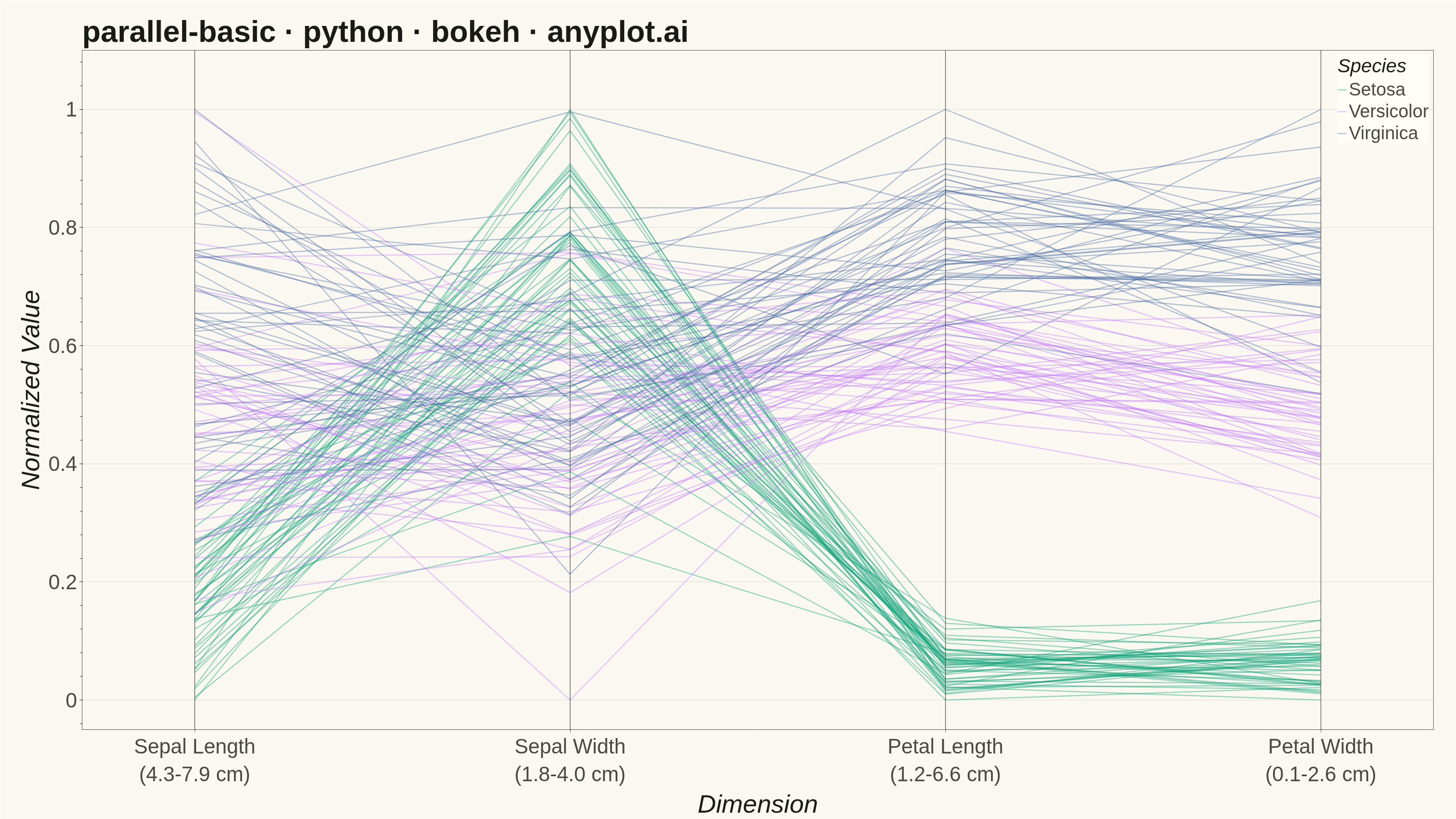
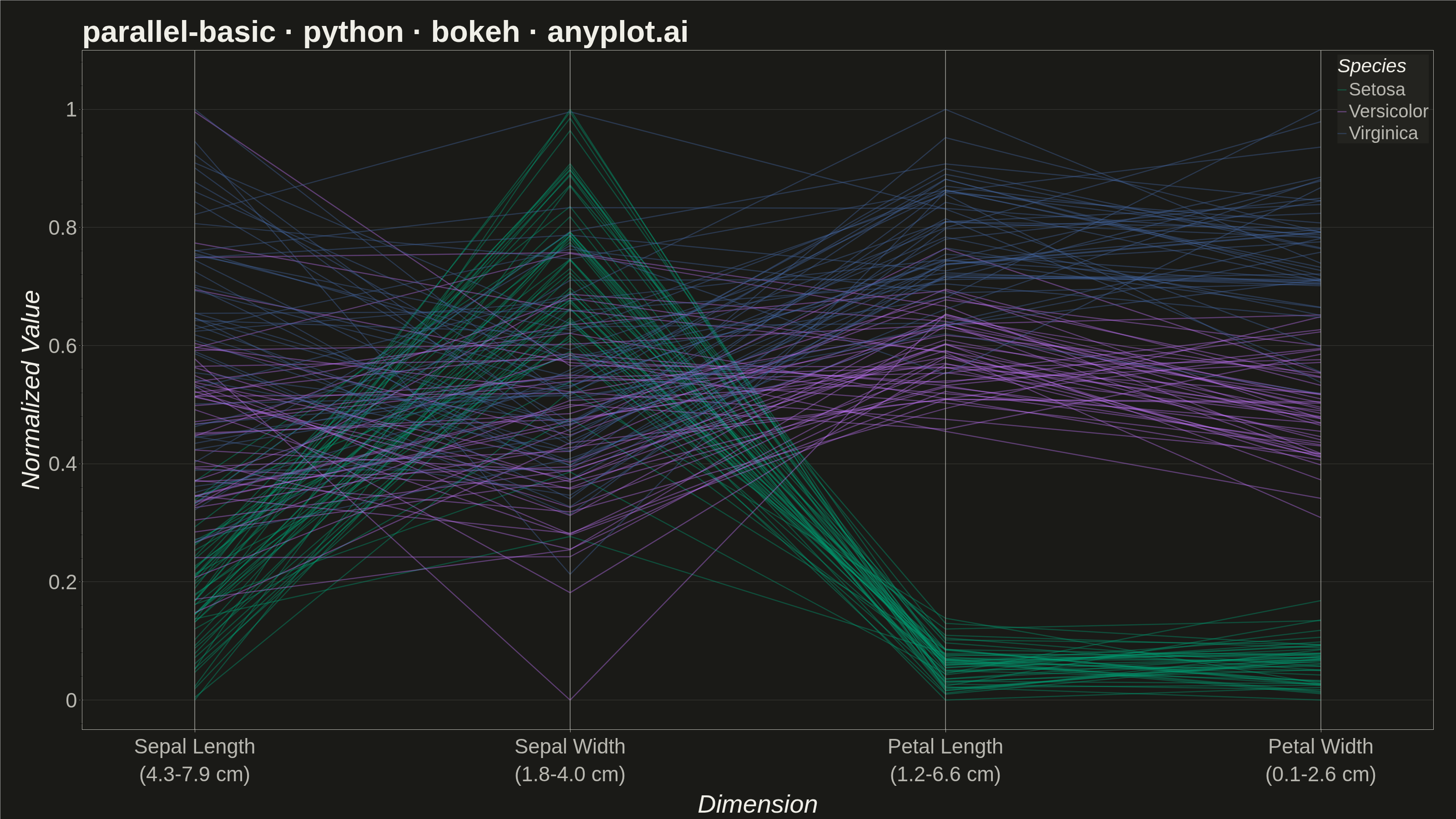
A parallel coordinates plot visualizes multivariate data by representing each variable as a vertical axis and each observation as a line connecting values across all axes. This technique is powerful for identifying patterns, clusters, and outliers in high-dimensional datasets where traditional 2D plots fall short. It enables simultaneous comparison of multiple variables for each data point.
""" anyplot.ai
parallel-basic: Basic Parallel Coordinates Plot
Library: bokeh 3.9.1 | Python 3.13.14
Quality: 94/100 | Updated: 2026-07-24
"""

import os
import sys
import time
from pathlib import Path


_script_dir = os.path.dirname(os.path.abspath(__file__))
sys.path = [p for p in sys.path if os.path.abspath(p or ".") != _script_dir]

import numpy as np
import pandas as pd
from bokeh.io import output_file, save
from bokeh.models import ColumnDataSource, HoverTool, Span
from bokeh.plotting import figure
from selenium import webdriver
from selenium.webdriver.chrome.options import Options


# Theme tokens (see prompts/default-style-guide.md "Theme-adaptive Chrome")
THEME = os.getenv("ANYPLOT_THEME", "light")
PAGE_BG = "#FAF8F1" if THEME == "light" else "#1A1A17"
ELEVATED_BG = "#FFFDF6" if THEME == "light" else "#242420"
INK = "#1A1A17" if THEME == "light" else "#F0EFE8"
INK_SOFT = "#4A4A44" if THEME == "light" else "#B8B7B0"

# Imprint palette (position 1 is always the first categorical series)
IMPRINT_PALETTE = ["#009E73", "#C475FD", "#4467A3", "#BD8233", "#AE3030", "#2ABCCD", "#954477", "#99B314"]

# Data - Iris-like dataset for multivariate demonstration
np.random.seed(42)

n_per_species = 50

# Setosa: small petals, moderate sepals
setosa = pd.DataFrame(
    {
        "sepal_length": np.random.normal(5.0, 0.35, n_per_species),
        "sepal_width": np.random.normal(3.4, 0.38, n_per_species),
        "petal_length": np.random.normal(1.5, 0.17, n_per_species),
        "petal_width": np.random.normal(0.25, 0.10, n_per_species),
        "species": "setosa",
    }
)

# Versicolor: medium everything
versicolor = pd.DataFrame(
    {
        "sepal_length": np.random.normal(5.9, 0.52, n_per_species),
        "sepal_width": np.random.normal(2.8, 0.31, n_per_species),
        "petal_length": np.random.normal(4.3, 0.47, n_per_species),
        "petal_width": np.random.normal(1.3, 0.20, n_per_species),
        "species": "versicolor",
    }
)

# Virginica: large petals and sepals
virginica = pd.DataFrame(
    {
        "sepal_length": np.random.normal(6.6, 0.64, n_per_species),
        "sepal_width": np.random.normal(3.0, 0.32, n_per_species),
        "petal_length": np.random.normal(5.5, 0.55, n_per_species),
        "petal_width": np.random.normal(2.0, 0.27, n_per_species),
        "species": "virginica",
    }
)

df = pd.concat([setosa, versicolor, virginica], ignore_index=True)

# Normalize numeric columns to [0, 1] for fair comparison across axes
numeric_cols = ["sepal_length", "sepal_width", "petal_length", "petal_width"]
df_norm = df.copy()
for col in numeric_cols:
    min_val = df[col].min()
    max_val = df[col].max()
    df_norm[col] = (df[col] - min_val) / (max_val - min_val)

# Colors by species (Imprint palette, canonical order)
species_order = ["setosa", "versicolor", "virginica"]
colors = dict(zip(species_order, IMPRINT_PALETTE[:3], strict=True))

# One multi-line source: each row of xs/ys is a single observation's polyline
x_coords = list(range(len(numeric_cols)))
source = ColumnDataSource(
    data={
        "xs": [x_coords] * len(df_norm),
        "ys": df_norm[numeric_cols].values.tolist(),
        "species": df_norm["species"].str.capitalize(),
        "color": [colors[s] for s in df_norm["species"]],
    }
)

# Create figure (3200x1800 px landscape canvas)
title = "parallel-basic · python · bokeh · anyplot.ai"
p = figure(
    width=3200,
    height=1800,
    title=title,
    x_axis_label="Dimension",
    y_axis_label="Normalized Value",
    x_range=(-0.3, 3.3),
    y_range=(-0.05, 1.10),
    toolbar_location=None,  # bokeh's default toolbar adds ~30-50px above the plot
    min_border_bottom=160,  # room for 34pt x-tick labels + 42pt x-axis label
    min_border_left=180,  # room for 34pt y-tick labels + 42pt y-axis label
    min_border_top=110,  # room for 50pt title
    min_border_right=50,
)

# Plot parallel coordinates - one polyline per observation, colored by species.
# line_alpha=0.4 (down from 0.5) eases the densest crossover region (Sepal Width)
# while still preserving the crossing pattern. muted_alpha lets a legend click
# isolate a single species - a bokeh-distinctive touch beyond the plain HoverTool.
renderer = p.multi_line(
    xs="xs",
    ys="ys",
    source=source,
    line_color="color",
    line_alpha=0.4,
    line_width=2.5,
    legend_field="species",
    muted_alpha=0.05,
)

# Hover shows which species a given line belongs to - bokeh's signature interactive feature
hover = HoverTool(renderers=[renderer], tooltips=[("Species", "@species")], line_policy="nearest")
p.add_tools(hover)

# Vertical axis line per dimension - bolder than the shared 0.15-alpha grid so
# each of the four parallel-coordinate axes reads as a distinct anchor line.
for x in x_coords:
    p.add_layout(Span(location=x, dimension="height", line_color=INK_SOFT, line_width=2, line_alpha=0.6))

p.legend.click_policy = "mute"
p.legend.title = "Species"
p.legend.location = "top_right"
p.legend.label_text_font_size = "30pt"
p.legend.title_text_font_size = "32pt"
p.legend.background_fill_color = ELEVATED_BG
p.legend.border_line_color = None
p.legend.label_text_color = INK_SOFT
p.legend.title_text_color = INK

# Custom x-axis labels with original scale ranges
axis_labels = [
    f"Sepal Length\n({df['sepal_length'].min():.1f}-{df['sepal_length'].max():.1f} cm)",
    f"Sepal Width\n({df['sepal_width'].min():.1f}-{df['sepal_width'].max():.1f} cm)",
    f"Petal Length\n({df['petal_length'].min():.1f}-{df['petal_length'].max():.1f} cm)",
    f"Petal Width\n({df['petal_width'].min():.1f}-{df['petal_width'].max():.1f} cm)",
]
p.xaxis.ticker = x_coords
p.xaxis.major_label_overrides = dict(enumerate(axis_labels))

# Text sizes and typography for 3200x1800 px canvas - helvetica throughout for
# a deliberate, publication-grade look rather than bokeh's default font stack
p.title.text_font = "helvetica"
p.title.text_font_size = "50pt"
p.xaxis.axis_label_text_font = "helvetica"
p.yaxis.axis_label_text_font = "helvetica"
p.xaxis.axis_label_text_font_size = "42pt"
p.yaxis.axis_label_text_font_size = "42pt"
p.xaxis.major_label_text_font = "helvetica"
p.yaxis.major_label_text_font = "helvetica"
p.xaxis.major_label_text_font_size = "34pt"
p.yaxis.major_label_text_font_size = "34pt"
p.legend.label_text_font = "helvetica"
p.legend.title_text_font = "helvetica"

# Theme-adaptive chrome
p.background_fill_color = PAGE_BG
p.border_fill_color = PAGE_BG
p.outline_line_color = INK_SOFT

p.title.text_color = INK
p.xaxis.axis_label_text_color = INK
p.yaxis.axis_label_text_color = INK
p.xaxis.major_label_text_color = INK_SOFT
p.yaxis.major_label_text_color = INK_SOFT
p.xaxis.axis_line_color = INK_SOFT
p.yaxis.axis_line_color = INK_SOFT
p.xaxis.major_tick_line_color = INK_SOFT
p.yaxis.major_tick_line_color = INK_SOFT

# Grid styling - subtle
p.xgrid.grid_line_color = INK
p.ygrid.grid_line_color = INK
p.xgrid.grid_line_alpha = 0.15
p.ygrid.grid_line_alpha = 0.15

# Save outputs - write HTML then screenshot with headless Chrome (bokeh's export_png
# is unreliable in this environment; see prompts/library/bokeh.md)
output_file(f"plot-{THEME}.html", title=title)
save(p)

W, H = 3200, 1800
opts = Options()
for arg in (
    "--headless=new",
    "--no-sandbox",
    "--disable-dev-shm-usage",
    "--disable-gpu",
    f"--window-size={W},{H}",
    "--hide-scrollbars",
):
    opts.add_argument(arg)
driver = webdriver.Chrome(options=opts)
driver.set_window_size(W, H)
driver.get(f"file://{Path(f'plot-{THEME}.html').resolve()}")
# Headless Chrome's --window-size sets the OUTER window (a phantom ~143px
# title bar eats into it even headless), so innerHeight ends up short of H.
# Override the viewport directly via CDP for an exact WxH capture.
driver.execute_cdp_cmd(
    "Emulation.setDeviceMetricsOverride", {"width": W, "height": H, "deviceScaleFactor": 1, "mobile": False}
)
time.sleep(3)  # let bokeh's JS render the canvas
driver.save_screenshot(f"plot-{THEME}.png")
driver.quit()
Runnable source as JSON, for any HTTP client: https://api.anyplot.ai/specs/parallel-basic/bokeh/code. Any spec id and library id listed in llms-full.txt fit the same URL shape; every URL below is complete and callable.
{
  "spec_id": "parallel-basic",
  "language": "python",
  "library": "bokeh",
  "page": "https://anyplot.ai/parallel-basic/python/bokeh",
  "hub": "https://anyplot.ai/parallel-basic",
  "code_json": "https://api.anyplot.ai/specs/parallel-basic/bokeh/code",
  "spec_json": "https://api.anyplot.ai/specs/parallel-basic",
  "render_light_png": "https://storage.googleapis.com/anyplot-images/plots/parallel-basic/python/bokeh/plot-light.png",
  "render_dark_png": "https://storage.googleapis.com/anyplot-images/plots/parallel-basic/python/bokeh/plot-dark.png",
  "interactive_light_html": "https://storage.googleapis.com/anyplot-images/plots/parallel-basic/python/bokeh/plot-light.html",
  "interactive_dark_html": "https://storage.googleapis.com/anyplot-images/plots/parallel-basic/python/bokeh/plot-dark.html",
  "quality_score": 94.0,
  "license": "MIT",
  "guide": "https://anyplot.ai/llms.txt"
}
Part of Basic Parallel Coordinates Plot on anyplot.ai.