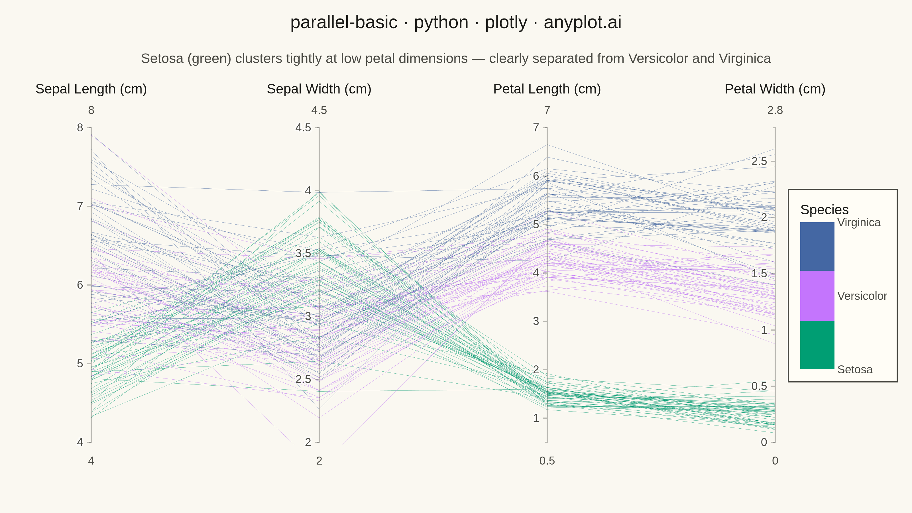
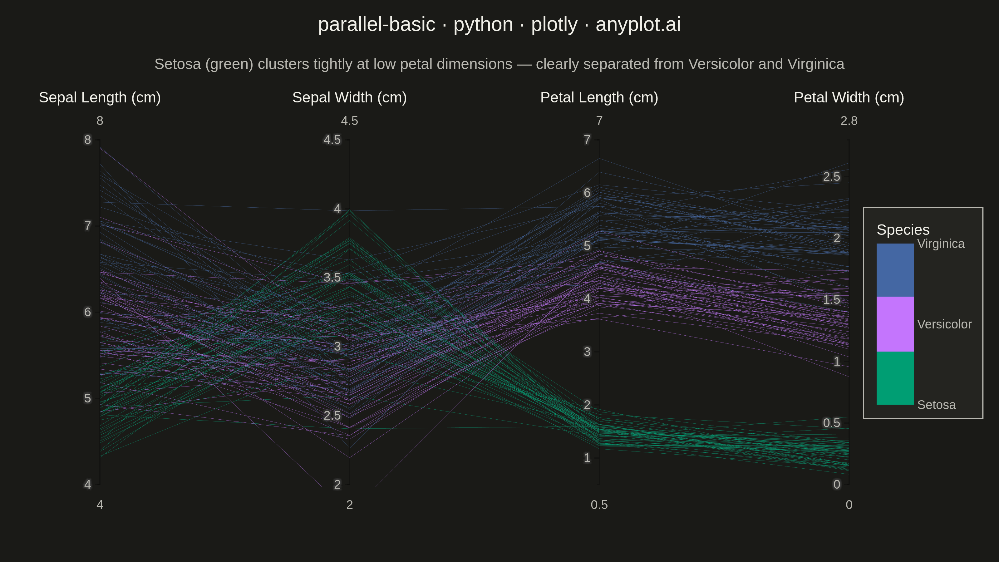
A parallel coordinates plot visualizes multivariate data by representing each variable as a vertical axis and each observation as a line connecting values across all axes. This technique is powerful for identifying patterns, clusters, and outliers in high-dimensional datasets where traditional 2D plots fall short. It enables simultaneous comparison of multiple variables for each data point.
""" anyplot.ai
parallel-basic: Basic Parallel Coordinates Plot
Library: plotly 6.9.0 | Python 3.13.14
Quality: 89/100 | Updated: 2026-07-24
"""

import os

import numpy as np
import pandas as pd
import plotly.graph_objects as go


# Theme tokens
THEME = os.getenv("ANYPLOT_THEME", "light")
PAGE_BG = "#FAF8F1" if THEME == "light" else "#1A1A17"
ELEVATED_BG = "#FFFDF6" if THEME == "light" else "#242420"
INK = "#1A1A17" if THEME == "light" else "#F0EFE8"
INK_SOFT = "#4A4A44" if THEME == "light" else "#B8B7B0"


# Imprint palette discrete colorscale: Setosa=#009E73, Versicolor=#C475FD, Virginica=#4467A3
# Kept fully opaque (no alpha blending) so hues stay pixel-identical between themes —
# translucency would composite against PAGE_BG, which differs between light and dark.
IMPRINT_COLORSCALE = [
    [0.0, "#009E73"],
    [0.33, "#009E73"],
    [0.33, "#C475FD"],
    [0.67, "#C475FD"],
    [0.67, "#4467A3"],
    [1.0, "#4467A3"],
]

# Data - Iris-like dataset for multivariate demonstration
np.random.seed(42)
n_per_species = 50

setosa = pd.DataFrame(
    {
        "sepal_length": np.random.normal(5.0, 0.35, n_per_species),
        "sepal_width": np.random.normal(3.4, 0.38, n_per_species),
        "petal_length": np.random.normal(1.5, 0.17, n_per_species),
        "petal_width": np.random.normal(0.25, 0.11, n_per_species),
        "species": "setosa",
    }
)

versicolor = pd.DataFrame(
    {
        "sepal_length": np.random.normal(5.9, 0.52, n_per_species),
        "sepal_width": np.random.normal(2.8, 0.31, n_per_species),
        "petal_length": np.random.normal(4.3, 0.47, n_per_species),
        "petal_width": np.random.normal(1.3, 0.20, n_per_species),
        "species": "versicolor",
    }
)

virginica = pd.DataFrame(
    {
        "sepal_length": np.random.normal(6.6, 0.64, n_per_species),
        "sepal_width": np.random.normal(3.0, 0.32, n_per_species),
        "petal_length": np.random.normal(5.6, 0.55, n_per_species),
        "petal_width": np.random.normal(2.0, 0.27, n_per_species),
        "species": "virginica",
    }
)

df = pd.concat([setosa, versicolor, virginica], ignore_index=True)
species_map = {"setosa": 0, "versicolor": 1, "virginica": 2}
df["species_code"] = df["species"].map(species_map)

# Plot
fig = go.Figure(
    data=go.Parcoords(
        line={
            "color": df["species_code"],
            "colorscale": IMPRINT_COLORSCALE,
            "showscale": True,
            "cmin": 0,
            "cmax": 2,
            "colorbar": {
                "title": {"text": "Species", "font": {"size": 12, "color": INK}},
                "tickvals": [0, 1, 2],
                "ticktext": ["Setosa", "Versicolor", "Virginica"],
                "tickfont": {"size": 10, "color": INK_SOFT},
                "len": 0.6,
                "y": 0.5,
                "bgcolor": ELEVATED_BG,
                "bordercolor": INK_SOFT,
                "borderwidth": 1,
            },
        },
        dimensions=[
            {"label": "Sepal Length (cm)", "values": df["sepal_length"], "range": [4, 8]},
            {"label": "Sepal Width (cm)", "values": df["sepal_width"], "range": [2, 4.5]},
            {"label": "Petal Length (cm)", "values": df["petal_length"], "range": [0.5, 7]},
            {"label": "Petal Width (cm)", "values": df["petal_width"], "range": [0, 2.8]},
        ],
        labelfont={"size": 12, "color": INK},
        tickfont={"size": 10, "color": INK_SOFT},
        rangefont={"size": 10, "color": INK_SOFT},
    )
)

fig.update_layout(
    autosize=False,
    width=800,
    height=450,
    title={
        "text": "parallel-basic · python · plotly · anyplot.ai",
        "subtitle": {
            "text": "Setosa (green) clusters tightly at low petal dimensions"
            " — clearly separated from Versicolor and Virginica",
            "font": {"size": 12, "color": INK_SOFT},
        },
        "font": {"size": 16, "color": INK},
        "x": 0.5,
        "xanchor": "center",
        "y": 0.97,
    },
    paper_bgcolor=PAGE_BG,
    plot_bgcolor=PAGE_BG,
    font={"color": INK},
    margin={"l": 80, "r": 110, "t": 110, "b": 60},
)

# Save
fig.write_image(f"plot-{THEME}.png", width=800, height=450, scale=4)
fig.write_html(f"plot-{THEME}.html", include_plotlyjs="cdn")
Runnable source as JSON, for any HTTP client: https://api.anyplot.ai/specs/parallel-basic/plotly/code. Any spec id and library id listed in llms-full.txt fit the same URL shape; every URL below is complete and callable.
{
  "spec_id": "parallel-basic",
  "language": "python",
  "library": "plotly",
  "page": "https://anyplot.ai/parallel-basic/python/plotly",
  "hub": "https://anyplot.ai/parallel-basic",
  "code_json": "https://api.anyplot.ai/specs/parallel-basic/plotly/code",
  "spec_json": "https://api.anyplot.ai/specs/parallel-basic",
  "render_light_png": "https://storage.googleapis.com/anyplot-images/plots/parallel-basic/python/plotly/plot-light.png",
  "render_dark_png": "https://storage.googleapis.com/anyplot-images/plots/parallel-basic/python/plotly/plot-dark.png",
  "interactive_light_html": "https://storage.googleapis.com/anyplot-images/plots/parallel-basic/python/plotly/plot-light.html",
  "interactive_dark_html": "https://storage.googleapis.com/anyplot-images/plots/parallel-basic/python/plotly/plot-dark.html",
  "quality_score": 89.0,
  "license": "MIT",
  "guide": "https://anyplot.ai/llms.txt"
}
Part of Basic Parallel Coordinates Plot on anyplot.ai.