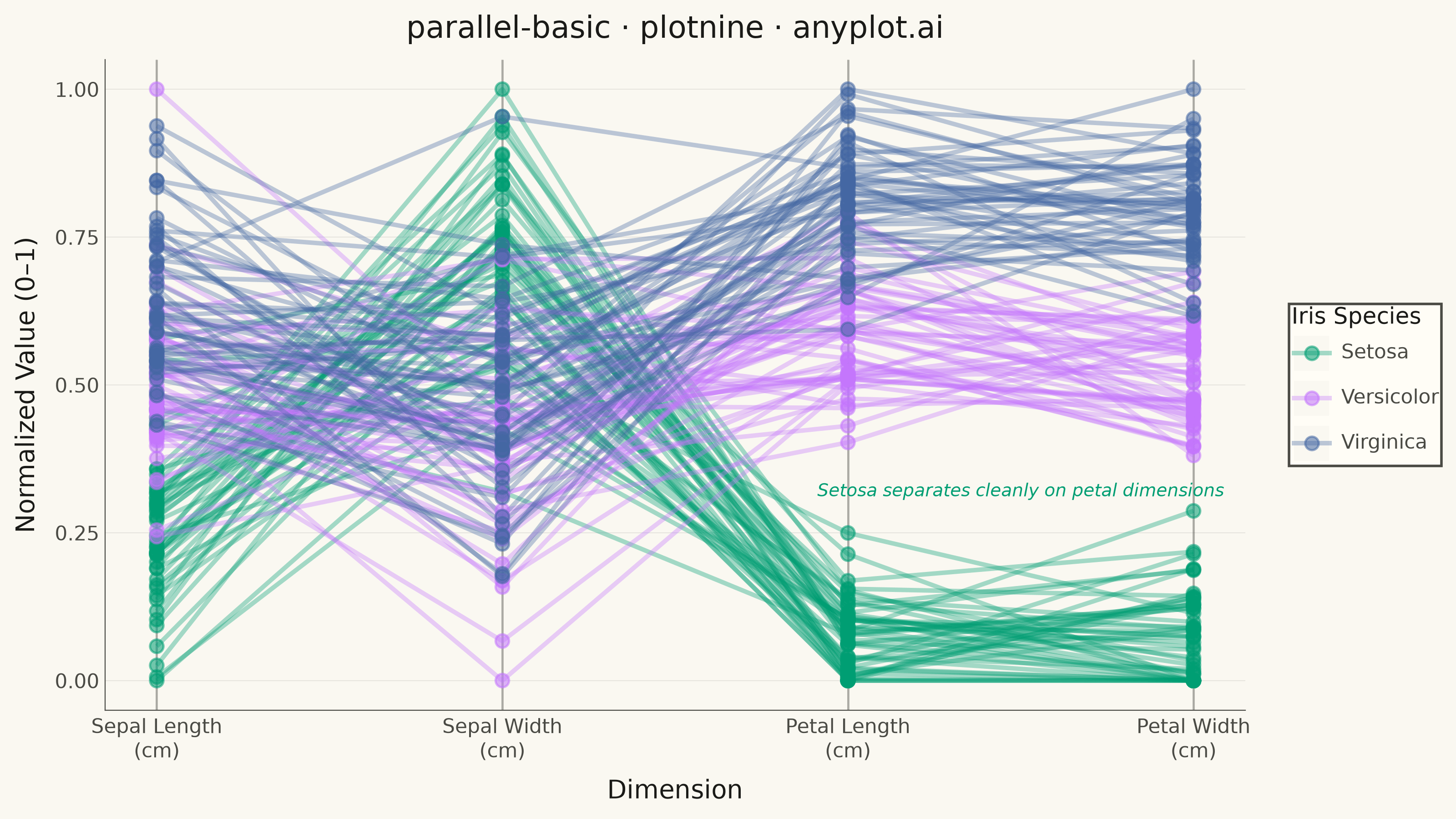
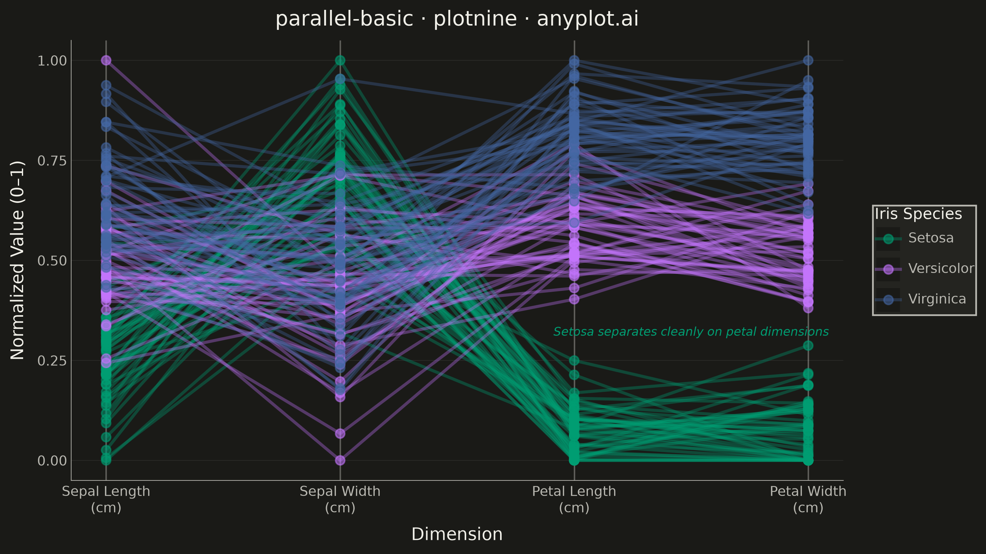
A parallel coordinates plot visualizes multivariate data by representing each variable as a vertical axis and each observation as a line connecting values across all axes. This technique is powerful for identifying patterns, clusters, and outliers in high-dimensional datasets where traditional 2D plots fall short. It enables simultaneous comparison of multiple variables for each data point.
""" anyplot.ai
parallel-basic: Basic Parallel Coordinates Plot
Library: plotnine 0.15.7 | Python 3.13.14
Quality: 86/100 | Updated: 2026-07-24
"""

import os

import numpy as np
import pandas as pd
from plotnine import (
    aes,
    annotate,
    element_blank,
    element_line,
    element_rect,
    element_text,
    geom_line,
    geom_point,
    geom_vline,
    ggplot,
    labs,
    scale_color_manual,
    scale_x_continuous,
    theme,
    theme_minimal,
)


# Theme tokens
THEME = os.getenv("ANYPLOT_THEME", "light")
PAGE_BG = "#FAF8F1" if THEME == "light" else "#1A1A17"
ELEVATED_BG = "#FFFDF6" if THEME == "light" else "#242420"
INK = "#1A1A17" if THEME == "light" else "#F0EFE8"
INK_SOFT = "#4A4A44" if THEME == "light" else "#B8B7B0"

IMPRINT = ["#009E73", "#C475FD", "#4467A3", "#BD8233", "#AE3030", "#2ABCCD", "#954477"]

# Data — synthetic iris-like measurements, 50 samples per species (balanced)
np.random.seed(42)
n = 50
cov_setosa = np.diag([0.25, 0.09, 0.25, 0.04])
cov_versicol = np.diag([0.25, 0.09, 0.25, 0.04])
cov_virginica = np.diag([0.25, 0.09, 0.25, 0.04])
setosa = np.random.multivariate_normal([5.01, 3.42, 1.46, 0.24], cov_setosa, size=n)
versicol = np.random.multivariate_normal([5.94, 2.77, 4.26, 1.33], cov_versicol, size=n)
virginica = np.random.multivariate_normal([6.59, 2.97, 5.55, 2.03], cov_virginica, size=n)

cols = ["sepal_length", "sepal_width", "petal_length", "petal_width"]
df = pd.DataFrame(np.vstack([setosa, versicol, virginica]), columns=cols)
df["species"] = ["Setosa"] * n + ["Versicolor"] * n + ["Virginica"] * n
df["id"] = range(len(df))

# Clip to realistic ranges
df["sepal_length"] = df["sepal_length"].clip(4.0, 8.5)
df["sepal_width"] = df["sepal_width"].clip(2.0, 4.5)
df["petal_length"] = df["petal_length"].clip(1.0, 7.0)
df["petal_width"] = df["petal_width"].clip(0.1, 2.8)

# Normalize each dimension to 0–1 scale for fair comparison
dimensions = ["sepal_length", "sepal_width", "petal_length", "petal_width"]
df_norm = df.copy()
for col in dimensions:
    df_norm[col] = (df[col] - df[col].min()) / (df[col].max() - df[col].min())

# Transform to long format for parallel coordinates
df_long = pd.melt(df_norm, id_vars=["id", "species"], value_vars=dimensions, var_name="dimension", value_name="value")
dim_map = {dim: i for i, dim in enumerate(dimensions)}
df_long["dim_num"] = df_long["dimension"].map(dim_map)

# Imprint palette colors — first series always #009E73
species_order = ["Setosa", "Versicolor", "Virginica"]
colors = {sp: IMPRINT[i] for i, sp in enumerate(species_order)}

# Plot
plot = (
    ggplot(df_long, aes(x="dim_num", y="value", group="id", color="species"))
    + geom_vline(xintercept=list(range(len(dimensions))), color=INK_SOFT, size=0.5, alpha=0.4)
    + geom_line(alpha=0.35, size=1.0)
    + geom_point(size=2.5, alpha=0.55)
    + annotate(
        "text",
        x=2.5,
        y=0.32,
        label="Setosa separates cleanly on petal dimensions",
        color=IMPRINT[0],
        size=7,
        ha="center",
        fontstyle="italic",
    )
    + scale_color_manual(values=colors, breaks=species_order)
    + scale_x_continuous(
        breaks=list(range(len(dimensions))),
        labels=["Sepal Length\n(cm)", "Sepal Width\n(cm)", "Petal Length\n(cm)", "Petal Width\n(cm)"],
    )
    + labs(
        x="Dimension", y="Normalized Value (0–1)", title="parallel-basic · plotnine · anyplot.ai", color="Iris Species"
    )
    + theme_minimal()
    + theme(
        figure_size=(8, 4.5),
        plot_background=element_rect(fill=PAGE_BG, color=PAGE_BG),
        panel_background=element_rect(fill=PAGE_BG),
        panel_border=element_blank(),
        panel_grid_major=element_line(color=INK, size=0.3, alpha=0.10),
        panel_grid_minor=element_blank(),
        axis_title=element_text(color=INK, size=10),
        axis_text=element_text(color=INK_SOFT, size=8),
        axis_line=element_line(color=INK_SOFT, size=0.4),
        plot_title=element_text(color=INK, size=12),
        legend_background=element_rect(fill=ELEVATED_BG, color=INK_SOFT),
        legend_text=element_text(color=INK_SOFT, size=8),
        legend_title=element_text(color=INK, size=9),
        text=element_text(size=8),
    )
)

# Save
plot.save(f"plot-{THEME}.png", dpi=400, width=8, height=4.5, units="in", verbose=False)
Runnable source as JSON, for any HTTP client: https://api.anyplot.ai/specs/parallel-basic/plotnine/code. Any spec id and library id listed in llms-full.txt fit the same URL shape; every URL below is complete and callable.
{
  "spec_id": "parallel-basic",
  "language": "python",
  "library": "plotnine",
  "page": "https://anyplot.ai/parallel-basic/python/plotnine",
  "hub": "https://anyplot.ai/parallel-basic",
  "code_json": "https://api.anyplot.ai/specs/parallel-basic/plotnine/code",
  "spec_json": "https://api.anyplot.ai/specs/parallel-basic",
  "render_light_png": "https://storage.googleapis.com/anyplot-images/plots/parallel-basic/python/plotnine/plot-light.png",
  "render_dark_png": "https://storage.googleapis.com/anyplot-images/plots/parallel-basic/python/plotnine/plot-dark.png",
  "quality_score": 86.0,
  "license": "MIT",
  "guide": "https://anyplot.ai/llms.txt"
}
Part of Basic Parallel Coordinates Plot on anyplot.ai.