The same plot in 14 other libraries — Python: Altair, Bokeh, lets-plot, Matplotlib, Plotly, plotnine, Pygal, Seaborn; Julia: Makie.jl; JavaScript: Chart.js, D3.js, Apache ECharts, Highcharts, MUI X Charts. Compare all 15 side by side: Basic Parallel Coordinates Plot in Python, R, Julia and JavaScript.
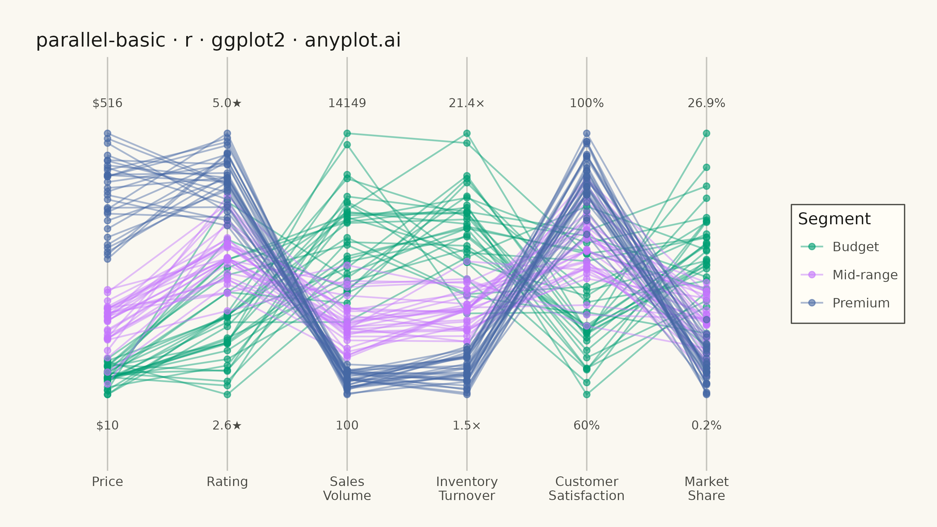
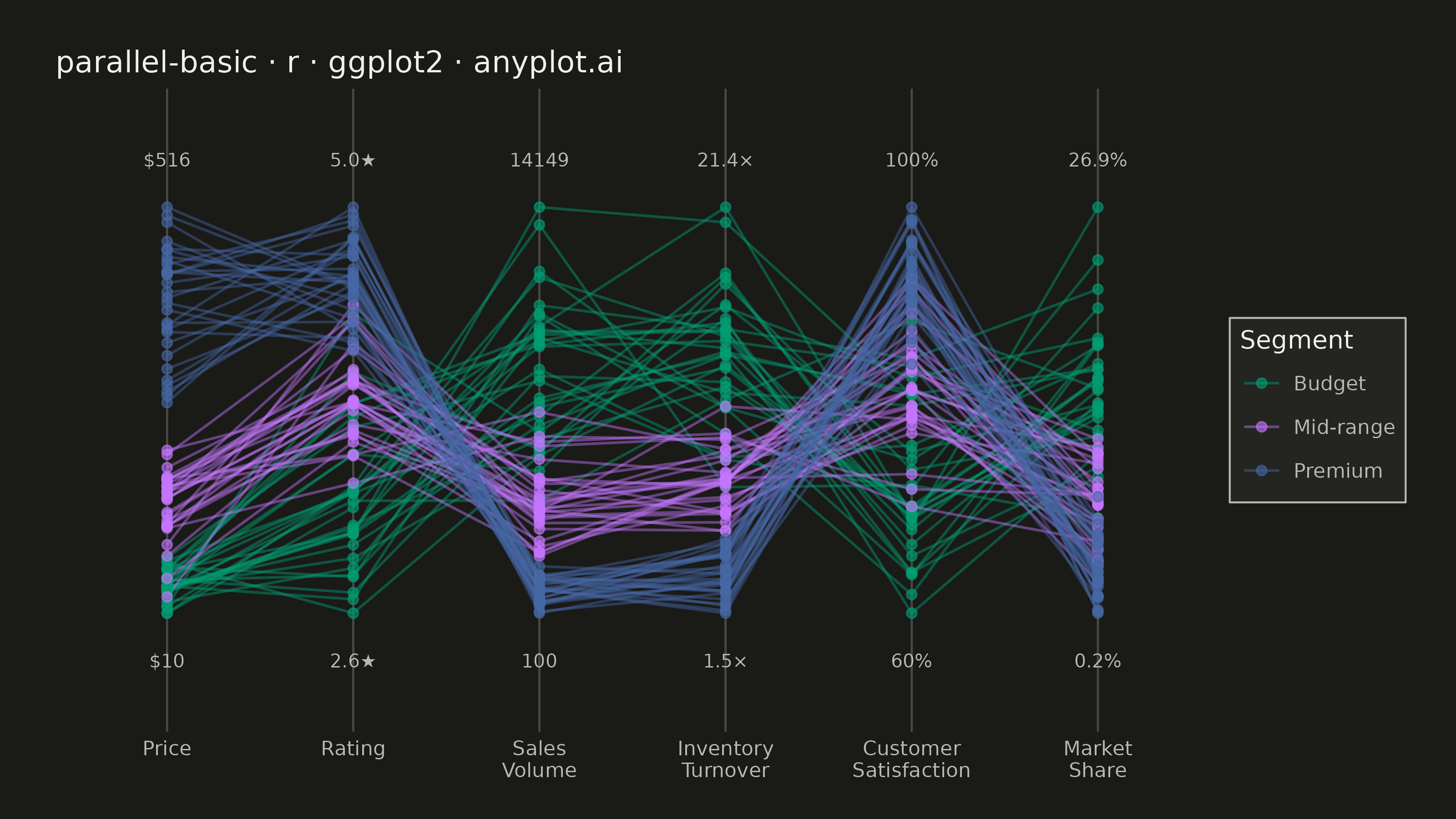
A parallel coordinates plot visualizes multivariate data by representing each variable as a vertical axis and each observation as a line connecting values across all axes. This technique is powerful for identifying patterns, clusters, and outliers in high-dimensional datasets where traditional 2D plots fall short. It enables simultaneous comparison of multiple variables for each data point.
#' anyplot.ai
#' parallel-basic: Basic Parallel Coordinates Plot
#' Library: ggplot2 3.5.1 | R 4.4.1
#' Quality: 90/100 | Created: 2026-07-24

library(ggplot2)
library(dplyr)
library(tidyr)
library(ragg)

set.seed(42)

# --- Theme tokens -------------------------------------------------------
THEME       <- Sys.getenv("ANYPLOT_THEME", "light")
PAGE_BG     <- if (THEME == "light") "#FAF8F1" else "#1A1A17"
ELEVATED_BG <- if (THEME == "light") "#FFFDF6" else "#242420"
INK         <- if (THEME == "light") "#1A1A17" else "#F0EFE8"
INK_SOFT    <- if (THEME == "light") "#4A4A44" else "#B8B7B0"
IMPRINT_PALETTE <- c(
  "#009E73", # 1 - brand green
  "#C475FD", # 2 - lavender
  "#4467A3"  # 3 - blue
)

# --- Data -----------------------------------------------------------------
# Product feature comparison across 6 metrics for 3 market segments.
n_per_segment  <- 30
segment_levels <- c("Budget", "Mid-range", "Premium")
seg_idx        <- rep(1:3, each = n_per_segment)
n              <- length(seg_idx)

price                  <- pmax(rnorm(n, c(45, 150, 380)[seg_idx], c(15, 40, 90)[seg_idx]), 10)
rating                 <- pmin(pmax(rnorm(n, c(3.3, 4.0, 4.6)[seg_idx], c(0.4, 0.3, 0.25)[seg_idx]), 1), 5)
sales_volume           <- pmax(rnorm(n, c(9000, 4000, 900)[seg_idx], c(2500, 1500, 400)[seg_idx]), 100)
inventory_turnover     <- pmax(rnorm(n, c(14, 8, 3.5)[seg_idx], c(3, 2, 1.2)[seg_idx]), 1)
customer_satisfaction  <- pmin(pmax(rnorm(n, c(72, 84, 93)[seg_idx], c(7, 6, 4)[seg_idx]), 40), 100)
market_share           <- pmax(rnorm(n, c(15, 8, 3)[seg_idx], c(4, 3, 1.5)[seg_idx]), 0.2)

dimension_cols <- c("Price", "Rating", "Sales Volume", "Inventory Turnover",
                     "Customer Satisfaction", "Market Share")

products <- tibble::tibble(
  id                       = seq_len(n),
  category                 = factor(segment_levels[seg_idx], levels = segment_levels),
  Price                    = price,
  Rating                   = rating,
  `Sales Volume`           = sales_volume,
  `Inventory Turnover`     = inventory_turnover,
  `Customer Satisfaction`  = customer_satisfaction,
  `Market Share`           = market_share
)

# Min-max normalize each dimension to [0, 1] so all axes are comparable.
products_norm <- products %>%
  mutate(across(all_of(dimension_cols), ~ (. - min(.)) / (max(.) - min(.)), .names = "{.col}_norm"))

products_long <- products_norm %>%
  select(id, category, ends_with("_norm")) %>%
  pivot_longer(cols = ends_with("_norm"), names_to = "dimension", values_to = "value") %>%
  mutate(
    dimension = sub("_norm$", "", dimension),
    dimension = factor(dimension, levels = dimension_cols)
  )

# Original-scale min/max labels shown at each axis endpoint.
axis_fmt <- c(
  "Price"                 = "$%.0f",
  "Rating"                = "%.1f★",
  "Sales Volume"          = "%.0f",
  "Inventory Turnover"    = "%.1f×",
  "Customer Satisfaction" = "%.0f%%",
  "Market Share"          = "%.1f%%"
)
axis_range <- products %>%
  summarise(across(all_of(dimension_cols), list(min = min, max = max))) %>%
  pivot_longer(everything(), names_to = c("dimension", ".value"), names_pattern = "(.*)_(min|max)") %>%
  mutate(
    dimension = factor(dimension, levels = dimension_cols),
    x         = as.numeric(dimension),
    min_label = sprintf(axis_fmt[as.character(dimension)], min),
    max_label = sprintf(axis_fmt[as.character(dimension)], max)
  )

# --- Plot -------------------------------------------------------------------
anyplot_theme <- theme_minimal(base_size = 8) +
  theme(
    plot.background    = element_rect(fill = PAGE_BG, color = PAGE_BG),
    panel.background   = element_rect(fill = PAGE_BG, color = NA),
    panel.grid         = element_blank(),
    panel.border       = element_blank(),
    axis.line          = element_blank(),
    axis.ticks         = element_blank(),
    axis.text.y        = element_blank(),
    axis.title         = element_blank(),
    axis.text.x        = element_text(color = INK_SOFT, size = 8),
    plot.title         = element_text(color = INK, size = 12),
    legend.background  = element_rect(fill = ELEVATED_BG, color = INK_SOFT),
    legend.text        = element_text(color = INK_SOFT, size = 8),
    legend.title       = element_text(color = INK, size = 10)
  )

p <- ggplot() +
  geom_vline(
    data = axis_range, aes(xintercept = x),
    color = INK_SOFT, alpha = 0.3, linewidth = 0.4
  ) +
  geom_line(
    data = products_long,
    aes(x = dimension, y = value, group = id, color = category),
    alpha = 0.45, linewidth = 0.5
  ) +
  geom_point(
    data = products_long,
    aes(x = dimension, y = value, color = category),
    size = 1.5, alpha = 0.6
  ) +
  geom_text(
    data = axis_range, aes(x = x, y = -0.1, label = min_label),
    color = INK_SOFT, size = 2.6, vjust = 1
  ) +
  geom_text(
    data = axis_range, aes(x = x, y = 1.1, label = max_label),
    color = INK_SOFT, size = 2.6, vjust = 0
  ) +
  scale_color_manual(values = IMPRINT_PALETTE, name = "Segment") +
  scale_x_discrete(labels = function(x) gsub(" ", "\n", x), expand = expansion(add = 0.6)) +
  coord_cartesian(ylim = c(-0.22, 1.22), clip = "off") +
  labs(title = "parallel-basic · r · ggplot2 · anyplot.ai") +
  anyplot_theme +
  theme(plot.margin = margin(t = 20, r = 20, b = 15, l = 20))

# --- Save -------------------------------------------------------------------
ggsave(
  filename = sprintf("plot-%s.png", THEME),
  plot     = p,
  device   = ragg::agg_png,
  width    = 8,
  height   = 4.5,
  units    = "in",
  dpi      = 400
)
Runnable source as JSON, for any HTTP client: https://api.anyplot.ai/specs/parallel-basic/ggplot2/code. Any spec id and library id listed in llms-full.txt fit the same URL shape; every URL below is complete and callable.
{
  "spec_id": "parallel-basic",
  "language": "r",
  "library": "ggplot2",
  "page": "https://anyplot.ai/parallel-basic/r/ggplot2",
  "hub": "https://anyplot.ai/parallel-basic",
  "code_json": "https://api.anyplot.ai/specs/parallel-basic/ggplot2/code",
  "spec_json": "https://api.anyplot.ai/specs/parallel-basic",
  "render_light_png": "https://storage.googleapis.com/anyplot-images/plots/parallel-basic/r/ggplot2/plot-light.png",
  "render_dark_png": "https://storage.googleapis.com/anyplot-images/plots/parallel-basic/r/ggplot2/plot-dark.png",
  "quality_score": 90.0,
  "license": "MIT",
  "guide": "https://anyplot.ai/llms.txt"
}
Part of Basic Parallel Coordinates Plot on anyplot.ai.