The same plot in 14 other libraries — JavaScript: D3.js, Apache ECharts, Highcharts, MUI X Charts; Python: Altair, Bokeh, lets-plot, Matplotlib, Plotly, plotnine, Pygal, Seaborn; R: ggplot2; Julia: Makie.jl. Compare all 15 side by side: Probability-Probability (P-P) Plot in Python, R, Julia and JavaScript.
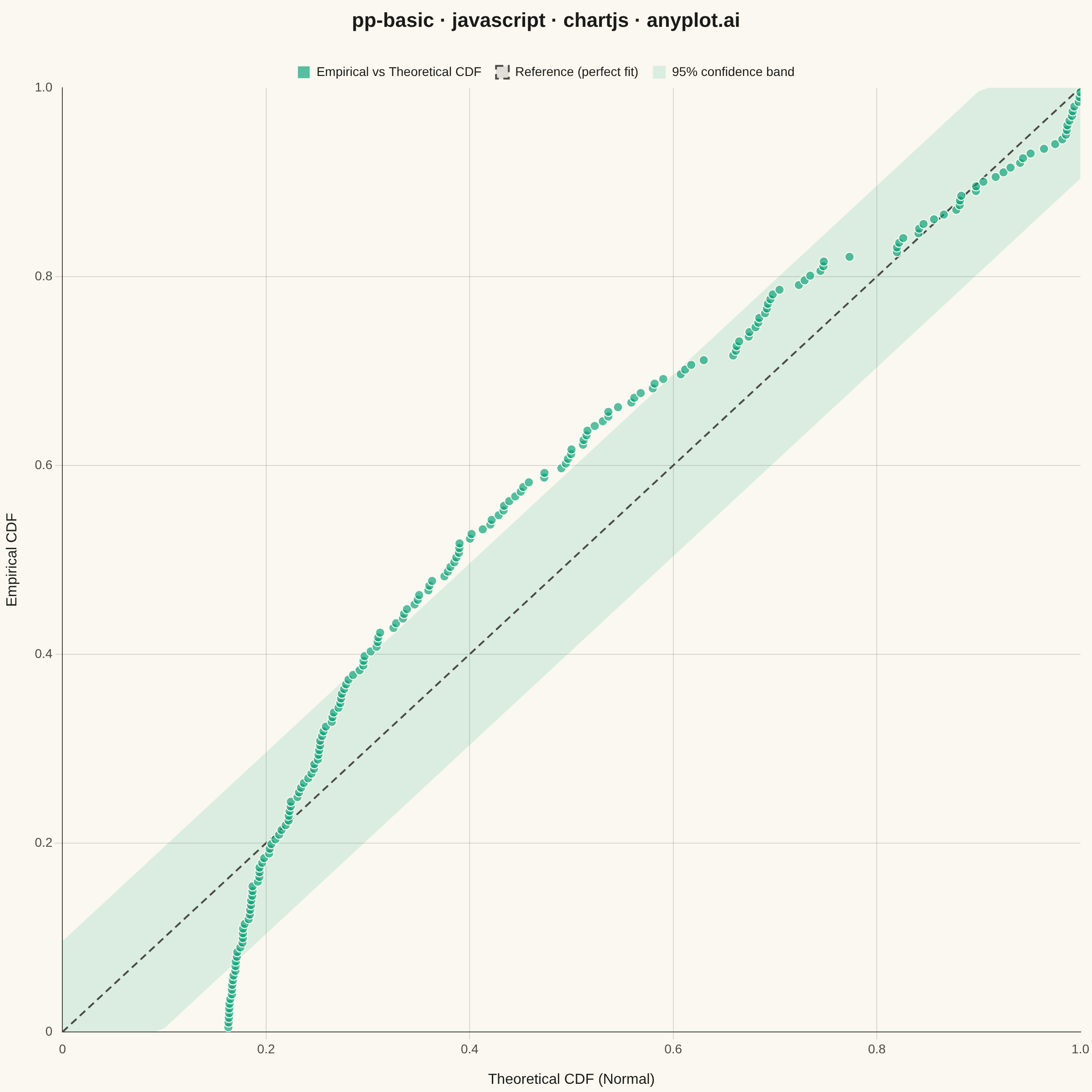
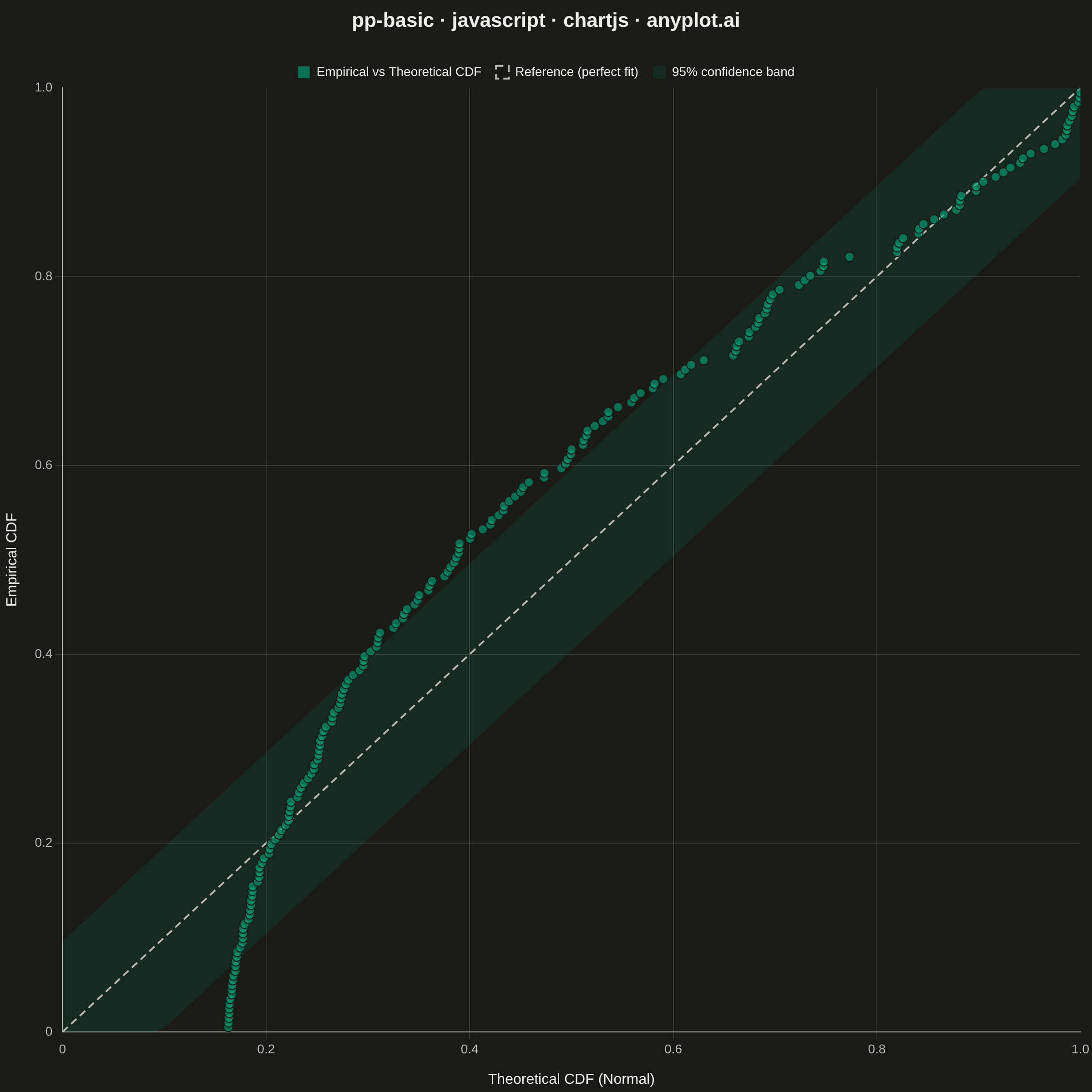
A diagnostic plot comparing the cumulative distribution function (CDF) of observed data against a theoretical distribution by plotting empirical CDF values against theoretical CDF values. Unlike Q-Q plots which compare quantiles, P-P plots compare cumulative probabilities on both axes (0 to 1), making them more sensitive to deviations in the center of the distribution. Points falling along the 45-degree diagonal indicate a good fit.
// anyplot.ai
// pp-basic: Probability-Probability (P-P) Plot
// Library: chartjs 4.4.7 | JavaScript 22.22.3
// Quality: 89/100 | Created: 2026-06-09
//# anyplot-orientation: square
const t = window.ANYPLOT_TOKENS;

// --- Data: 200 samples from a right-skewed distribution vs normal reference ---
// Deterministic LCG for reproducibility (no seeded Math.random in browser)
let seed = 987654321;
function lcg() {
  seed = (seed * 1664525 + 1013904223) >>> 0;
  return seed / 0x100000000;
}

function randn() {
  const u1 = Math.max(lcg(), 1e-10);
  const u2 = lcg();
  return Math.sqrt(-2 * Math.log(u1)) * Math.cos(2 * Math.PI * u2);
}

// 200 samples with slight right skew: z + 0.3*z^2 shifts mass rightward
const n = 200;
const rawData = Array.from({ length: n }, () => {
  const z = randn();
  return z + 0.3 * z * z;
});

// Sort ascending for empirical CDF
const sorted = [...rawData].sort((a, b) => a - b);

// Fit normal: sample mean and standard deviation
const mean = sorted.reduce((s, v) => s + v, 0) / n;
const std = Math.sqrt(sorted.reduce((s, v) => s + (v - mean) ** 2, 0) / n);

// Error function (Abramowitz & Stegun, max error ~1.5e-7)
function erf(x) {
  const sign = x >= 0 ? 1 : -1;
  const a = Math.abs(x);
  const t1 = 1 / (1 + 0.3275911 * a);
  const poly =
    (((1.061405429 * t1 - 1.453152027) * t1 + 1.421413741) * t1 - 0.284496736) * t1 + 0.254829592;
  return sign * (1 - poly * t1 * Math.exp(-a * a));
}

function normCDF(x, mu, sigma) {
  return 0.5 * (1 + erf((x - mu) / (sigma * Math.SQRT2)));
}

// P-P coordinates: (theoretical CDF, empirical CDF) for each sorted observation
const ppPoints = sorted.map((val, i) => ({
  x: normCDF(val, mean, std),
  y: (i + 1) / (n + 1), // Hazen plotting position
}));

// 45-degree reference line: perfect distributional fit
const refLine = [
  { x: 0, y: 0 },
  { x: 1, y: 1 },
];

// KS 95% confidence band: ±1.36/sqrt(n) from the diagonal
// Highlights whether S-curve deviation is statistically significant
const ksEps = 1.36 / Math.sqrt(n);
const xs = Array.from({ length: 101 }, (_, i) => i / 100);
const upperBand = xs.map((x) => ({ x, y: Math.min(1, x + ksEps) }));
const lowerBand = xs.map((x) => ({ x, y: Math.max(0, x - ksEps) }));

// --- Mount -----------------------------------------------------------------
const canvas = document.createElement("canvas");
document.getElementById("container").appendChild(canvas);

// Suppress grid lines at axis boundaries (value=0 and value=1) to achieve
// an L-shaped frame — removes the top and right box spines that Chart.js
// draws by default when tick grid lines coincide with the chart edge.
const innerGrid = (ctx) =>
  ctx.tick.value <= 0 || ctx.tick.value >= 1 ? "transparent" : t.grid;

// --- Chart -----------------------------------------------------------------
new Chart(canvas, {
  type: "scatter",
  data: {
    datasets: [
      {
        // Fill from upperBand to lowerBand (index +1) for the confidence envelope
        label: "95% confidence band",
        data: upperBand,
        type: "line",
        backgroundColor: t.palette[0] + "20",
        borderColor: "transparent",
        borderWidth: 0,
        pointRadius: 0,
        fill: "+1",
        tension: 0,
        order: 3,
      },
      {
        label: "_lower",
        data: lowerBand,
        type: "line",
        borderColor: "transparent",
        borderWidth: 0,
        pointRadius: 0,
        fill: false,
        tension: 0,
        order: 3,
      },
      {
        label: "Reference (perfect fit)",
        data: refLine,
        type: "line",
        borderColor: t.inkSoft,
        borderWidth: 2,
        borderDash: [8, 5],
        pointRadius: 0,
        fill: false,
        tension: 0,
        order: 2,
      },
      {
        label: "Empirical vs Theoretical CDF",
        data: ppPoints,
        backgroundColor: t.palette[0] + "a6",
        borderColor: t.pageBg,
        borderWidth: 1,
        pointRadius: 5,
        pointHoverRadius: 7,
        order: 1,
      },
    ],
  },
  options: {
    responsive: true,
    maintainAspectRatio: false,
    animation: false,
    plugins: {
      title: {
        display: true,
        text: "pp-basic · javascript · chartjs · anyplot.ai",
        color: t.ink,
        font: { size: 22, weight: "600" },
        padding: { top: 10, bottom: 20 },
      },
      legend: {
        labels: {
          color: t.ink,
          font: { size: 14 },
          boxWidth: 14,
          padding: 16,
          filter: (item) => !item.text.startsWith("_"),
        },
      },
    },
    scales: {
      x: {
        type: "linear",
        min: 0,
        max: 1,
        border: { display: true, color: t.inkSoft },
        ticks: {
          color: t.inkSoft,
          font: { size: 14 },
          maxTicksLimit: 6,
        },
        grid: { color: innerGrid },
        title: {
          display: true,
          text: "Theoretical CDF (Normal)",
          color: t.ink,
          font: { size: 16 },
          padding: { top: 12 },
        },
      },
      y: {
        type: "linear",
        min: 0,
        max: 1,
        border: { display: true, color: t.inkSoft },
        ticks: {
          color: t.inkSoft,
          font: { size: 14 },
          maxTicksLimit: 6,
        },
        grid: { color: innerGrid },
        title: {
          display: true,
          text: "Empirical CDF",
          color: t.ink,
          font: { size: 16 },
          padding: { bottom: 12 },
        },
      },
    },
  },
});
Runnable source as JSON, for any HTTP client: https://api.anyplot.ai/specs/pp-basic/chartjs/code. Any spec id and library id listed in llms-full.txt fit the same URL shape; every URL below is complete and callable.
{
  "spec_id": "pp-basic",
  "language": "javascript",
  "library": "chartjs",
  "page": "https://anyplot.ai/pp-basic/javascript/chartjs",
  "hub": "https://anyplot.ai/pp-basic",
  "code_json": "https://api.anyplot.ai/specs/pp-basic/chartjs/code",
  "spec_json": "https://api.anyplot.ai/specs/pp-basic",
  "render_light_png": "https://storage.googleapis.com/anyplot-images/plots/pp-basic/javascript/chartjs/plot-light.png",
  "render_dark_png": "https://storage.googleapis.com/anyplot-images/plots/pp-basic/javascript/chartjs/plot-dark.png",
  "interactive_light_html": "https://storage.googleapis.com/anyplot-images/plots/pp-basic/javascript/chartjs/plot-light.html",
  "interactive_dark_html": "https://storage.googleapis.com/anyplot-images/plots/pp-basic/javascript/chartjs/plot-dark.html",
  "quality_score": 89.0,
  "license": "MIT",
  "guide": "https://anyplot.ai/llms.txt"
}
Part of Probability-Probability (P-P) Plot on anyplot.ai.