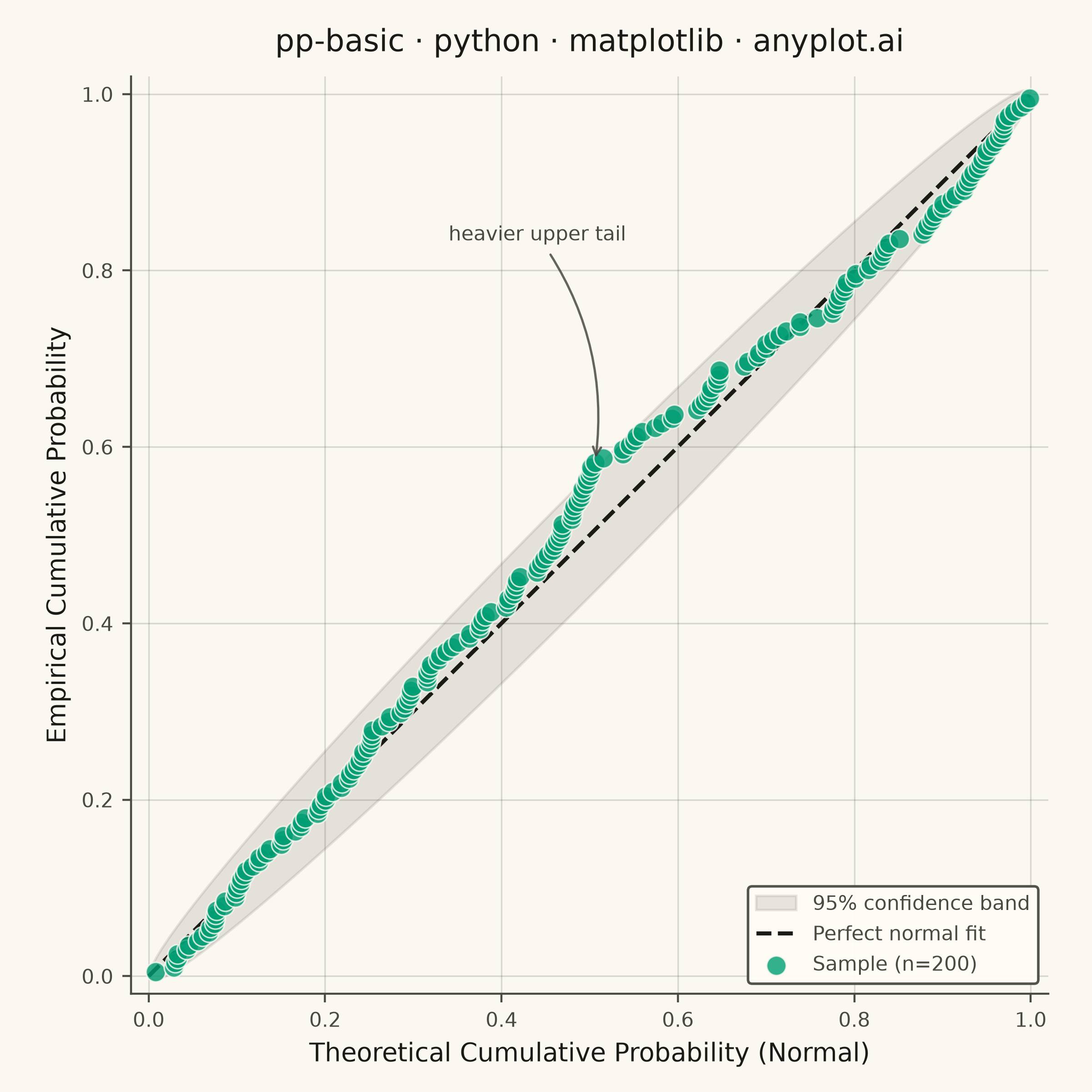
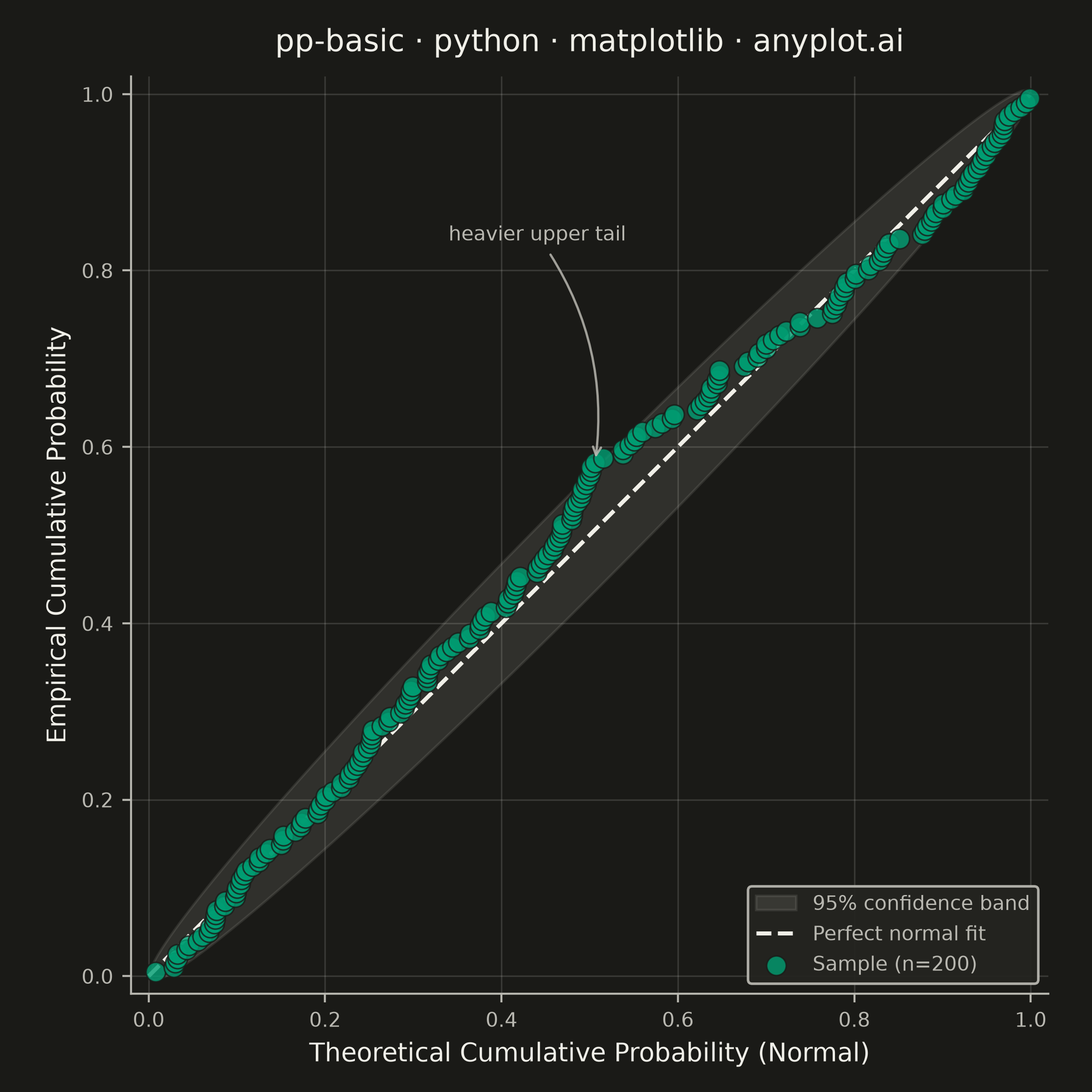
A diagnostic plot comparing the cumulative distribution function (CDF) of observed data against a theoretical distribution by plotting empirical CDF values against theoretical CDF values. Unlike Q-Q plots which compare quantiles, P-P plots compare cumulative probabilities on both axes (0 to 1), making them more sensitive to deviations in the center of the distribution. Points falling along the 45-degree diagonal indicate a good fit.
""" anyplot.ai
pp-basic: Probability-Probability (P-P) Plot
Library: matplotlib 3.11.0 | Python 3.13.13
Quality: 92/100 | Updated: 2026-06-16
"""

import os
import sys


# This file is named matplotlib.py; drop the script dir from sys.path so
# `import matplotlib` resolves to the installed package, not this module.
_script_dir = os.path.abspath(os.path.dirname(__file__))
sys.path = [p for p in sys.path if os.path.abspath(p or os.getcwd()) != _script_dir]
sys.modules.pop("matplotlib", None)

import matplotlib.pyplot as plt
import matplotlib.ticker as mticker
import numpy as np
from scipy.stats import norm


# Theme-adaptive chrome (see prompts/default-style-guide.md "Theme-adaptive Chrome")
THEME = os.getenv("ANYPLOT_THEME", "light")
PAGE_BG = "#FAF8F1" if THEME == "light" else "#1A1A17"
ELEVATED_BG = "#FFFDF6" if THEME == "light" else "#242420"
INK = "#1A1A17" if THEME == "light" else "#F0EFE8"
INK_SOFT = "#4A4A44" if THEME == "light" else "#B8B7B0"
INK_MUTED = "#6B6A63" if THEME == "light" else "#A8A79F"
BRAND = "#009E73"  # Imprint palette position 1 — always the first series

# Data — manufacturing quality control: bolt tensile strength (MPa)
# A small secondary-supplier batch creates a heavier upper tail, so the
# sample departs from normality in the classic P-P S-shape.
np.random.seed(42)
sample_size = 200
primary_batch = np.random.normal(loc=840, scale=35, size=160)
secondary_batch = np.random.normal(loc=910, scale=28, size=40)
tensile_strength = np.concatenate([primary_batch, secondary_batch])

observed_sorted = np.sort(tensile_strength)
empirical_cdf = np.arange(1, sample_size + 1) / (sample_size + 1)

mu, sigma = observed_sorted.mean(), observed_sorted.std(ddof=0)
theoretical_cdf = norm.cdf((observed_sorted - mu) / sigma)

# Plot — square canvas keeps the 45-degree diagonal meaningful (→ 2400×2400 px)
fig, ax = plt.subplots(figsize=(6, 6), dpi=400, facecolor=PAGE_BG)
ax.set_facecolor(PAGE_BG)

# 95% confidence band from order-statistic variance of the cumulative probabilities
band_x = np.linspace(0, 1, 200)
se = np.sqrt(band_x * (1 - band_x) / sample_size)
ax.fill_between(
    band_x, band_x - 1.96 * se, band_x + 1.96 * se, color=INK_MUTED, alpha=0.16, zorder=0, label="95% confidence band"
)

# Perfect-fit reference diagonal (neutral structural line)
ax.plot([0, 1], [0, 1], color=INK, linewidth=1.6, linestyle="--", zorder=1, label="Perfect normal fit")

# Empirical vs. theoretical cumulative probabilities
ax.scatter(
    theoretical_cdf,
    empirical_cdf,
    s=60,
    color=BRAND,
    alpha=0.8,
    edgecolors=PAGE_BG,
    linewidth=0.6,
    zorder=3,
    label="Sample (n=200)",
)

# Call out the S-shape: the secondary-supplier batch lifts the upper tail
# above the diagonal. Annotate the point of largest positive departure.
departure = empirical_cdf - theoretical_cdf
tail_idx = int(np.argmax(departure))
ax.annotate(
    "heavier upper tail",
    xy=(theoretical_cdf[tail_idx], empirical_cdf[tail_idx]),
    xytext=(0.34, 0.84),
    fontsize=8,
    color=INK_SOFT,
    ha="left",
    va="center",
    zorder=4,
    arrowprops={
        "arrowstyle": "->",
        "color": INK_SOFT,
        "linewidth": 0.9,
        "alpha": 0.85,
        "connectionstyle": "arc3,rad=-0.2",
    },
)

# Style
ax.set_xlabel("Theoretical Cumulative Probability (Normal)", fontsize=10, color=INK)
ax.set_ylabel("Empirical Cumulative Probability", fontsize=10, color=INK)
ax.set_title("pp-basic · python · matplotlib · anyplot.ai", fontsize=12, fontweight="medium", color=INK, pad=10)
ax.tick_params(axis="both", labelsize=8, colors=INK_SOFT)
ax.xaxis.set_major_locator(mticker.MultipleLocator(0.2))
ax.yaxis.set_major_locator(mticker.MultipleLocator(0.2))
ax.set_xlim(-0.02, 1.02)
ax.set_ylim(-0.02, 1.02)
ax.set_aspect("equal")

ax.spines["top"].set_visible(False)
ax.spines["right"].set_visible(False)
for s in ("left", "bottom"):
    ax.spines[s].set_color(INK_SOFT)
    ax.spines[s].set_linewidth(0.8)
ax.grid(True, alpha=0.15, linewidth=0.6, color=INK)

# Legend
leg = ax.legend(fontsize=8, loc="lower right", framealpha=0.95)
leg.get_frame().set_facecolor(ELEVATED_BG)
leg.get_frame().set_edgecolor(INK_SOFT)
for text in leg.get_texts():
    text.set_color(INK_SOFT)

fig.subplots_adjust(left=0.11, right=0.97, top=0.93, bottom=0.09)

# Save
plt.savefig(f"plot-{THEME}.png", dpi=400, facecolor=PAGE_BG)
Runnable source as JSON, for any HTTP client: https://api.anyplot.ai/specs/pp-basic/matplotlib/code. Any spec id and library id listed in llms-full.txt fit the same URL shape; every URL below is complete and callable.
{
  "spec_id": "pp-basic",
  "language": "python",
  "library": "matplotlib",
  "page": "https://anyplot.ai/pp-basic/python/matplotlib",
  "hub": "https://anyplot.ai/pp-basic",
  "code_json": "https://api.anyplot.ai/specs/pp-basic/matplotlib/code",
  "spec_json": "https://api.anyplot.ai/specs/pp-basic",
  "render_light_png": "https://storage.googleapis.com/anyplot-images/plots/pp-basic/python/matplotlib/plot-light.png",
  "render_dark_png": "https://storage.googleapis.com/anyplot-images/plots/pp-basic/python/matplotlib/plot-dark.png",
  "quality_score": 92.0,
  "license": "MIT",
  "guide": "https://anyplot.ai/llms.txt"
}
Part of Probability-Probability (P-P) Plot on anyplot.ai.