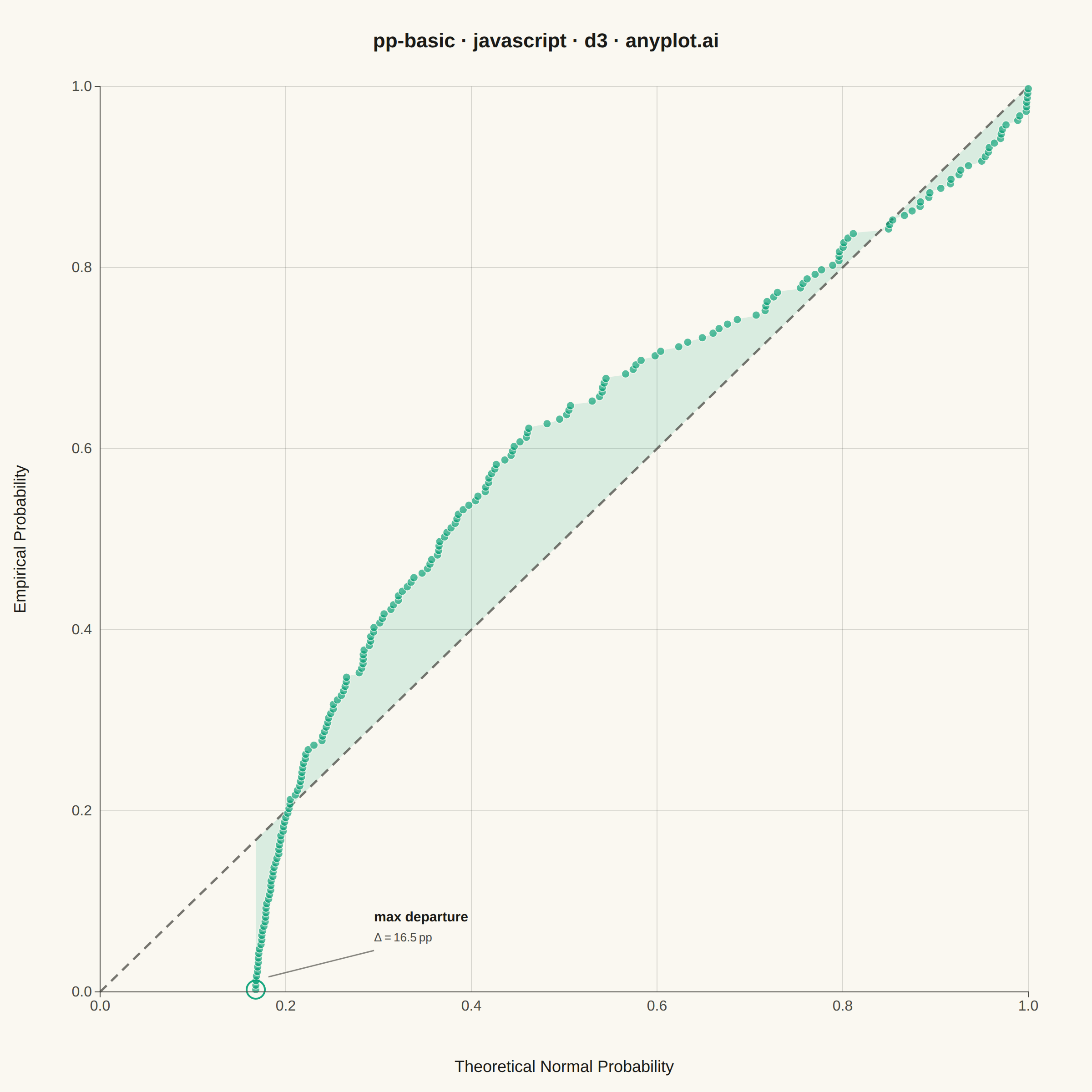
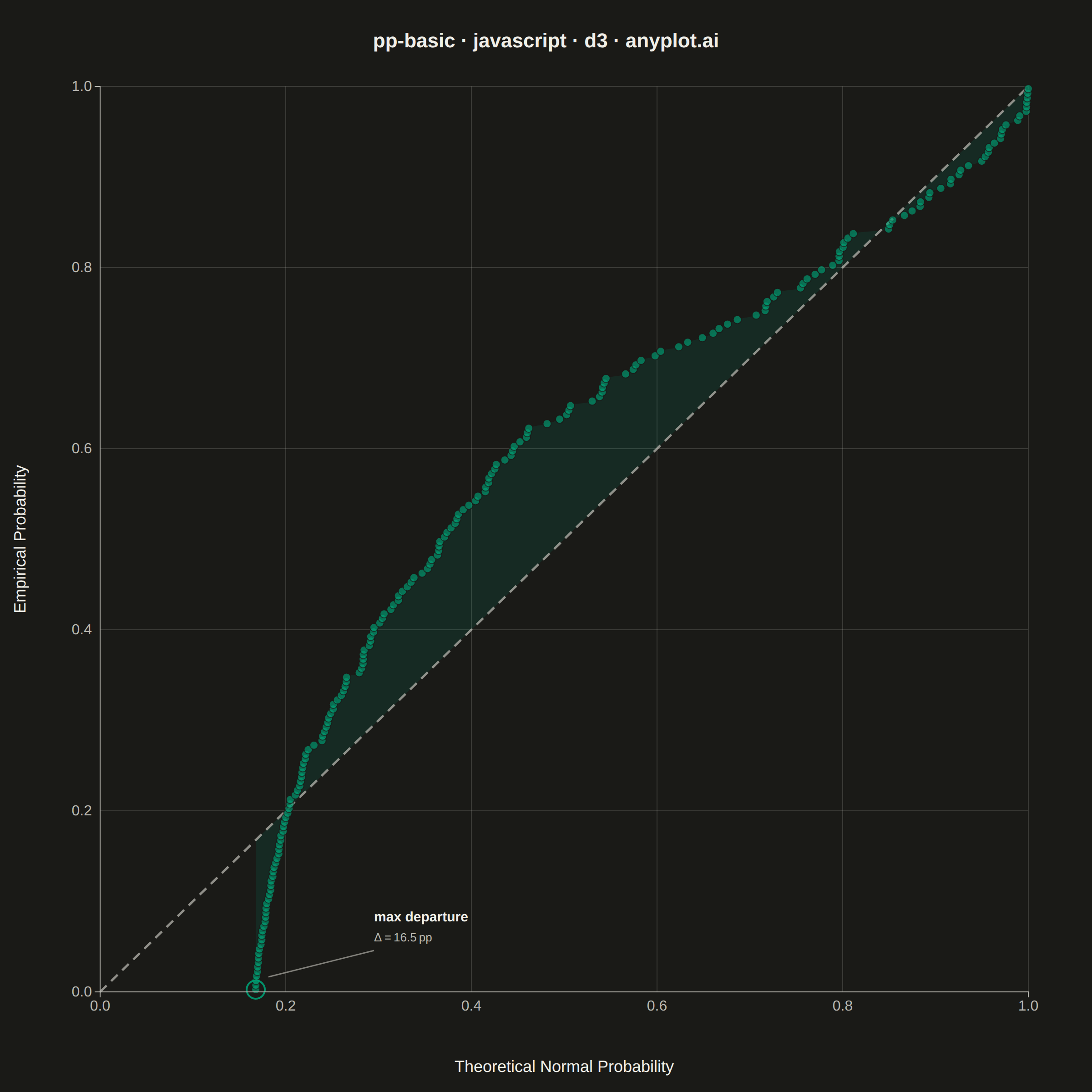
The same plot in 14 other libraries — JavaScript: Chart.js, Apache ECharts, Highcharts, MUI X Charts; Python: Altair, Bokeh, lets-plot, Matplotlib, Plotly, plotnine, Pygal, Seaborn; R: ggplot2; Julia: Makie.jl. Compare all 15 side by side: Probability-Probability (P-P) Plot in Python, R, Julia and JavaScript.
A diagnostic plot comparing the cumulative distribution function (CDF) of observed data against a theoretical distribution by plotting empirical CDF values against theoretical CDF values. Unlike Q-Q plots which compare quantiles, P-P plots compare cumulative probabilities on both axes (0 to 1), making them more sensitive to deviations in the center of the distribution. Points falling along the 45-degree diagonal indicate a good fit.
// anyplot.ai
// pp-basic: Probability-Probability (P-P) Plot
// Library: d3 7.9.0 | JavaScript 22.22.3
// Quality: 90/100 | Created: 2026-06-09

//# anyplot-orientation: square

const t = window.ANYPLOT_TOKENS;
const { width, height } = window.ANYPLOT_SIZE;

// --- Data (deterministic LCG, no browser RNG) ---
let seed = 42;
function rand() {
  seed = (Math.imul(seed, 1664525) + 1013904223) >>> 0;
  return seed / 4294967296;
}
function randn() {
  const u = rand() || 1e-10;
  const v = rand();
  return Math.sqrt(-2 * Math.log(u)) * Math.cos(2 * Math.PI * v);
}

// 200 samples from a slightly right-skewed distribution (normal + quadratic term)
// Context: manufacturing process measurements — testing normality assumption
const N = 200;
const raw = Array.from({ length: N }, () => {
  const z = randn();
  return z + 0.45 * z * z - 0.45; // right-skewed, bias-corrected
});

// Fit normal parameters to the sample
const sampleMean = raw.reduce((a, b) => a + b, 0) / N;
const sampleStd = Math.sqrt(raw.reduce((s, x) => s + (x - sampleMean) ** 2, 0) / (N - 1));

// Sort and compute empirical CDF (Hazen plotting position: (i + 0.5) / N)
const sorted = [...raw].sort((a, b) => a - b);
const empirical = sorted.map((_, i) => (i + 0.5) / N);

// Normal CDF via error function approximation (Abramowitz & Stegun 7.1.26)
function erf(z) {
  const a1 = 0.254829592,
    a2 = -0.284496736,
    a3 = 1.421413741;
  const a4 = -1.453152027,
    a5 = 1.061405429,
    q = 0.3275911;
  const sign = z < 0 ? -1 : 1;
  const ta = 1 / (1 + q * Math.abs(z));
  const y = 1 - (((((a5 * ta + a4) * ta + a3) * ta + a2) * ta + a1) * ta) * Math.exp(-z * z);
  return sign * y;
}
function normCDF(x, mu, sigma) {
  return 0.5 * (1 + erf((x - mu) / (sigma * Math.SQRT2)));
}

const theoretical = sorted.map((val) => normCDF(val, sampleMean, sampleStd));
const points = theoretical.map((th, i) => ({ th, em: empirical[i] }));

// Max absolute departure from the diagonal — the key diagnostic insight
const maxDevIdx = points.reduce(
  (best, p, i) => (Math.abs(p.em - p.th) > Math.abs(points[best].em - points[best].th) ? i : best),
  0,
);
const mdp = points[maxDevIdx];

// --- Layout ---
const margin = { top: 95, right: 70, bottom: 110, left: 110 };
const iw = width - margin.left - margin.right;
const ih = height - margin.top - margin.bottom;

const svg = d3
  .select("#container")
  .append("svg")
  .attr("width", width)
  .attr("height", height);

// Clip path — keeps deviation band and trend line inside plot bounds
svg
  .append("defs")
  .append("clipPath")
  .attr("id", "pp-clip")
  .append("rect")
  .attr("width", iw)
  .attr("height", ih);

const g = svg.append("g").attr("transform", `translate(${margin.left},${margin.top})`);

// --- Scales ---
const x = d3.scaleLinear().domain([0, 1]).range([0, iw]);
const y = d3.scaleLinear().domain([0, 1]).range([ih, 0]);

// --- Gridlines (both axes for scatter) ---
g.append("g")
  .selectAll("line")
  .data(x.ticks(5))
  .join("line")
  .attr("x1", (d) => x(d))
  .attr("x2", (d) => x(d))
  .attr("y1", 0)
  .attr("y2", ih)
  .attr("stroke", t.grid)
  .attr("stroke-width", 1);

g.append("g")
  .selectAll("line")
  .data(y.ticks(5))
  .join("line")
  .attr("x1", 0)
  .attr("x2", iw)
  .attr("y1", (d) => y(d))
  .attr("y2", (d) => y(d))
  .attr("stroke", t.grid)
  .attr("stroke-width", 1);

// --- Deviation band: d3.area between empirical curve and 45° diagonal ---
// Fills the departure region so the S-curve story is immediately visible
const areaGen = d3
  .area()
  .x((d) => x(d.th))
  .y0((d) => y(d.th)) // baseline: perfect-fit diagonal
  .y1((d) => y(d.em)) // actual: empirical CDF
  .curve(d3.curveMonotoneX);

g.append("path")
  .datum(points)
  .attr("d", areaGen)
  .attr("clip-path", "url(#pp-clip)")
  .attr("fill", t.palette[0])
  .attr("fill-opacity", 0.13)
  .attr("stroke", "none");

// --- 45-degree reference line (perfect fit) ---
g.append("line")
  .attr("x1", x(0))
  .attr("y1", y(0))
  .attr("x2", x(1))
  .attr("y2", y(1))
  .attr("stroke", t.inkSoft)
  .attr("stroke-width", 2.5)
  .attr("stroke-dasharray", "10,7")
  .attr("opacity", 0.75);

// --- Data points ---
g.selectAll("circle")
  .data(points)
  .join("circle")
  .attr("cx", (d) => x(d.th))
  .attr("cy", (d) => y(d.em))
  .attr("r", 4.5)
  .attr("fill", t.palette[0])
  .attr("opacity", 0.65)
  .attr("stroke", t.pageBg)
  .attr("stroke-width", 1);

// --- Highlight ring at maximum departure point ---
const mdpPx = x(mdp.th);
const mdpPy = y(mdp.em);

g.append("circle")
  .attr("cx", mdpPx)
  .attr("cy", mdpPy)
  .attr("r", 10)
  .attr("fill", "none")
  .attr("stroke", t.palette[0])
  .attr("stroke-width", 2)
  .attr("opacity", 0.9);

// --- Annotation: callout for maximum departure ---
const goRight = mdpPx < iw / 2;
const goUp = mdpPy >= ih / 3;
const aX = goRight ? mdpPx + 130 : mdpPx - 130;
const aY = goUp ? mdpPy - 75 : mdpPy + 75;
const anchor = goRight ? "start" : "end";
const connX = goRight ? mdpPx + 14 : mdpPx - 14;
const connY = goUp ? mdpPy - 14 : mdpPy + 14;

g.append("line")
  .attr("x1", connX)
  .attr("y1", connY)
  .attr("x2", aX)
  .attr("y2", aY + (goUp ? 32 : -32))
  .attr("stroke", t.inkSoft)
  .attr("stroke-width", 1.5)
  .attr("opacity", 0.65);

g.append("text")
  .attr("x", aX)
  .attr("y", aY)
  .attr("text-anchor", anchor)
  .attr("fill", t.ink)
  .style("font-size", "15px")
  .style("font-weight", "600")
  .text("max departure");

g.append("text")
  .attr("x", aX)
  .attr("y", aY + 22)
  .attr("text-anchor", anchor)
  .attr("fill", t.inkSoft)
  .style("font-size", "13px")
  .text(`Δ = ${(Math.abs(mdp.em - mdp.th) * 100).toFixed(1)} pp`);

// --- Axes ---
const xAxis = g
  .append("g")
  .attr("transform", `translate(0,${ih})`)
  .call(d3.axisBottom(x).ticks(5).tickFormat(d3.format(".1f")));

const yAxis = g.append("g").call(d3.axisLeft(y).ticks(5).tickFormat(d3.format(".1f")));

for (const ax of [xAxis, yAxis]) {
  ax.selectAll("text").attr("fill", t.inkSoft).style("font-size", "16px");
  ax.select(".domain").attr("stroke", t.inkSoft);
  ax.selectAll(".tick line").remove();
}

// --- Axis labels ---
svg
  .append("text")
  .attr("x", margin.left + iw / 2)
  .attr("y", height - 22)
  .attr("text-anchor", "middle")
  .attr("fill", t.ink)
  .style("font-size", "18px")
  .text("Theoretical Normal Probability");

svg
  .append("text")
  .attr("transform", "rotate(-90)")
  .attr("x", -(margin.top + ih / 2))
  .attr("y", 28)
  .attr("text-anchor", "middle")
  .attr("fill", t.ink)
  .style("font-size", "18px")
  .text("Empirical Probability");

// --- Title ---
svg
  .append("text")
  .attr("x", width / 2)
  .attr("y", 52)
  .attr("text-anchor", "middle")
  .attr("fill", t.ink)
  .style("font-size", "22px")
  .style("font-weight", "600")
  .text("pp-basic · javascript · d3 · anyplot.ai");
Runnable source as JSON, for any HTTP client: https://api.anyplot.ai/specs/pp-basic/d3/code. Any spec id and library id listed in llms-full.txt fit the same URL shape; every URL below is complete and callable.
{
  "spec_id": "pp-basic",
  "language": "javascript",
  "library": "d3",
  "page": "https://anyplot.ai/pp-basic/javascript/d3",
  "hub": "https://anyplot.ai/pp-basic",
  "code_json": "https://api.anyplot.ai/specs/pp-basic/d3/code",
  "spec_json": "https://api.anyplot.ai/specs/pp-basic",
  "render_light_png": "https://storage.googleapis.com/anyplot-images/plots/pp-basic/javascript/d3/plot-light.png",
  "render_dark_png": "https://storage.googleapis.com/anyplot-images/plots/pp-basic/javascript/d3/plot-dark.png",
  "interactive_light_html": "https://storage.googleapis.com/anyplot-images/plots/pp-basic/javascript/d3/plot-light.html",
  "interactive_dark_html": "https://storage.googleapis.com/anyplot-images/plots/pp-basic/javascript/d3/plot-dark.html",
  "quality_score": 90.0,
  "license": "MIT",
  "guide": "https://anyplot.ai/llms.txt"
}
Part of Probability-Probability (P-P) Plot on anyplot.ai.