The same plot in 14 other libraries — Python: Altair, Bokeh, lets-plot, Matplotlib, Plotly, plotnine, Pygal, Seaborn; R: ggplot2; JavaScript: Chart.js, D3.js, Apache ECharts, Highcharts, MUI X Charts. Compare all 15 side by side: Probability-Probability (P-P) Plot in Python, R, Julia and JavaScript.
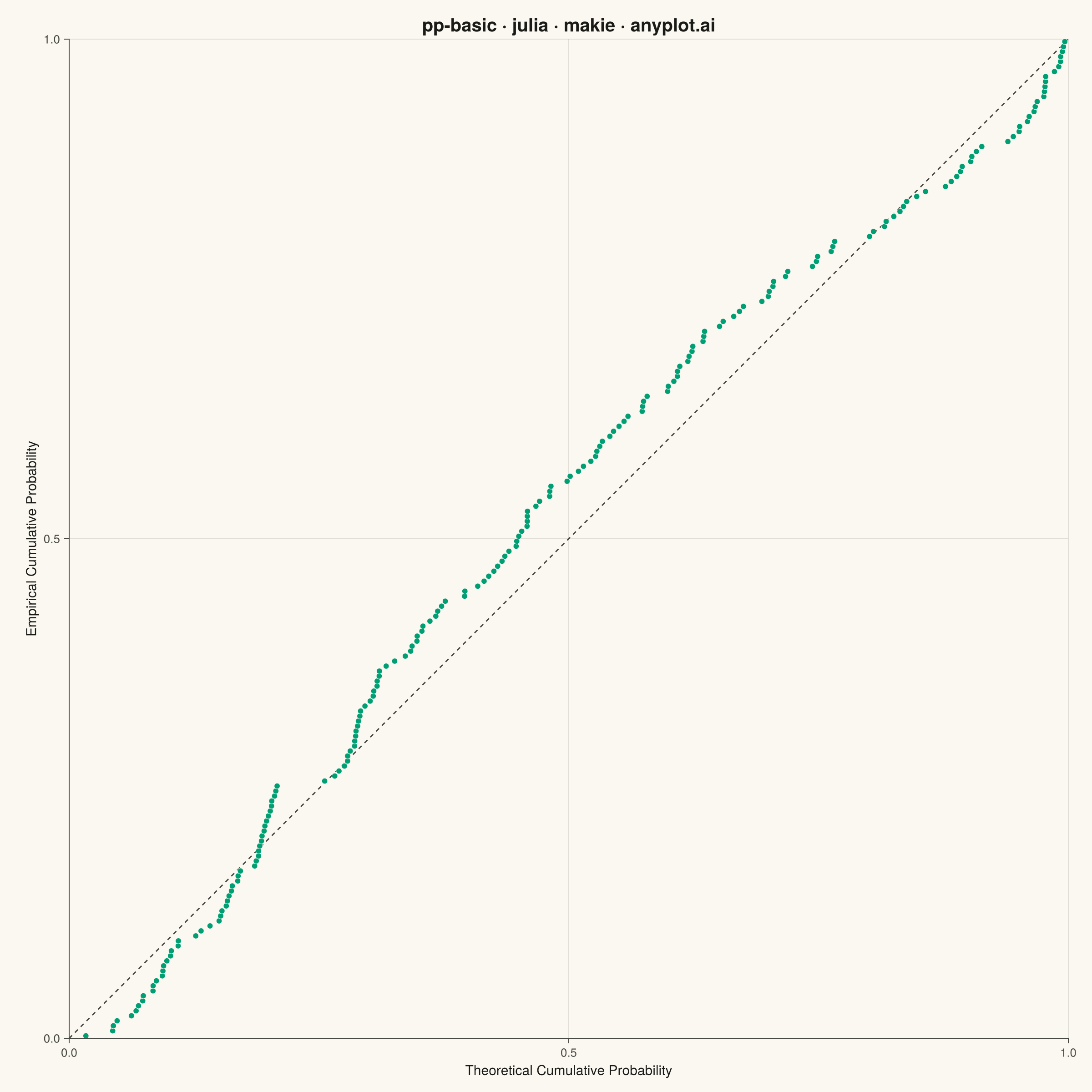
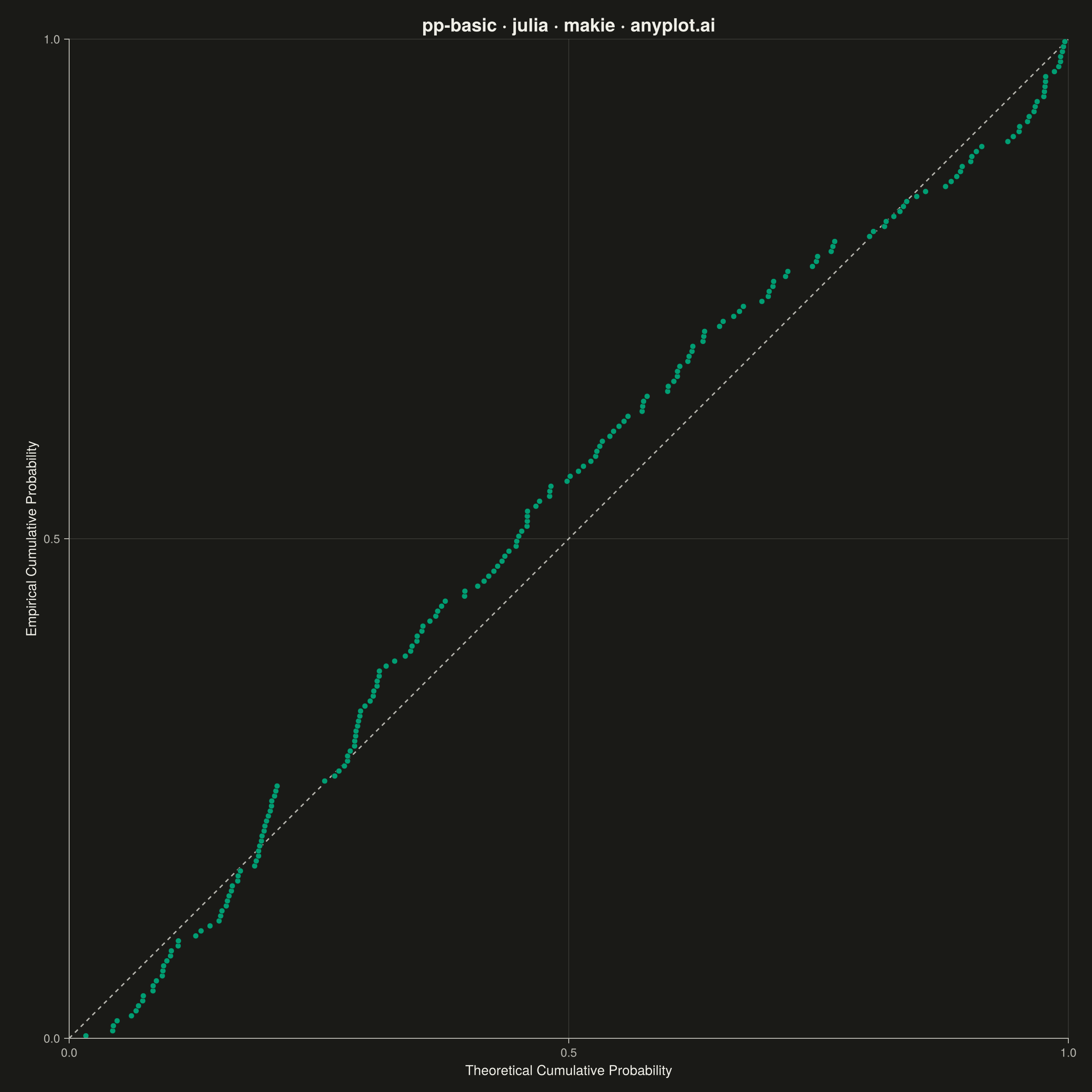
A diagnostic plot comparing the cumulative distribution function (CDF) of observed data against a theoretical distribution by plotting empirical CDF values against theoretical CDF values. Unlike Q-Q plots which compare quantiles, P-P plots compare cumulative probabilities on both axes (0 to 1), making them more sensitive to deviations in the center of the distribution. Points falling along the 45-degree diagonal indicate a good fit.
# anyplot.ai
# pp-basic: Probability-Probability (P-P) Plot
# Library: makie 0.22.10 | Julia 1.11.9
# Quality: 87/100 | Created: 2026-06-09

using CairoMakie
using ColorSchemes
using Colors
using Random
using Statistics

Random.seed!(42)

# Theme tokens
const THEME    = get(ENV, "ANYPLOT_THEME", "light")
const PAGE_BG  = THEME == "light" ? colorant"#FAF8F1" : colorant"#1A1A17"
const INK      = THEME == "light" ? colorant"#1A1A17" : colorant"#F0EFE8"
const INK_SOFT = THEME == "light" ? colorant"#4A4A44" : colorant"#B8B7B0"

const ANYPLOT_SEQ = cgrad([colorant"#009E73", colorant"#4467A3"])

# Data — process measurements (coating thickness, micrometers) with a right-skewed tail
# 85% from a normal base distribution, 15% with a positive boost → slightly right-skewed
n = 200
base_measurements = 50.0 .+ 8.0 .* randn(n)
boost_flags       = Float64.(rand(n) .< 0.15)
boost_amounts     = 20.0 .+ 5.0 .* abs.(randn(n))
coating_thickness = base_measurements .+ boost_flags .* boost_amounts

# Standardise to zero mean, unit variance for P-P comparison against N(0,1)
μ_fit    = mean(coating_thickness)
σ_fit    = std(coating_thickness)
z_scores = (coating_thickness .- μ_fit) ./ σ_fit

# Sort and compute empirical CDF (Hazen plotting positions: (i − 0.5) / n)
sorted_z      = sort(z_scores)
empirical_cdf = [(i - 0.5) / n for i in 1:n]

# Theoretical normal CDF — Abramowitz & Stegun (1964) rational approximation 26.2.17
# Maximum absolute error ≤ 7.5e-8; no external packages required.
abs_z     = abs.(sorted_z)
t_coeff   = 1.0 ./ (1.0 .+ 0.2316419 .* abs_z)
poly_val  = t_coeff .* (0.319381530 .+ t_coeff .* (
            -0.356563782 .+ t_coeff .* (
             1.781477937 .+ t_coeff .* (
            -1.821255978 .+ t_coeff .* 1.330274429))))
p_upper   = 1.0 .- (1.0 / sqrt(2π)) .* exp.(-abs_z .^ 2 ./ 2.0) .* poly_val
theoretical_cdf = ifelse.(sorted_z .>= 0.0, p_upper, 1.0 .- p_upper)

# Deviation from reference diagonal — key insight: S-curve departure from normality
dev     = abs.(empirical_cdf .- theoretical_cdf)
max_dev = maximum(dev)

# 95% KS confidence band half-width (D_α = 1.36 / √n)
delta  = 1.36 / sqrt(n)
xs_vec = collect(range(0.0, 1.0, length=200))

# Figure — square canvas (P-P plots use equal 0–1 probability axes)
fig = Figure(
    size            = (1200, 1200),
    fontsize        = 14,
    backgroundcolor = PAGE_BG,
)

ax = Axis(
    fig[1, 1];
    title             = "pp-basic · julia · makie · anyplot.ai",
    titlesize         = 28,
    titlecolor        = INK,
    xlabel            = "Theoretical Cumulative Probability",
    ylabel            = "Empirical Cumulative Probability",
    xlabelsize        = 20,
    ylabelsize        = 20,
    xticklabelsize    = 16,
    yticklabelsize    = 16,
    xlabelcolor       = INK,
    ylabelcolor       = INK,
    xticklabelcolor   = INK_SOFT,
    yticklabelcolor   = INK_SOFT,
    xtickcolor        = INK_SOFT,
    ytickcolor        = INK_SOFT,
    backgroundcolor   = PAGE_BG,
    topspinevisible   = false,
    rightspinevisible = false,
    leftspinecolor    = INK_SOFT,
    bottomspinecolor  = INK_SOFT,
    xgridcolor        = RGBAf(INK.r, INK.g, INK.b, 0.12),
    ygridcolor        = RGBAf(INK.r, INK.g, INK.b, 0.12),
    xminorgridvisible = false,
    yminorgridvisible = false,
    aspect            = AxisAspect(1),
    limits            = (0.0, 1.0, 0.0, 1.0),
)

# 95% KS confidence envelope — defines acceptance region around the diagonal
band!(ax, xs_vec, clamp.(xs_vec .- delta, 0.0, 1.0), clamp.(xs_vec .+ delta, 0.0, 1.0);
    color = RGBAf(INK.r, INK.g, INK.b, 0.07),
)

# Reference diagonal — perfect distributional fit
lines!(ax, [0.0, 1.0], [0.0, 1.0];
    color     = INK_SOFT,
    linewidth = 1.5,
    linestyle = :dash,
)

# P-P scatter — points colored by absolute deviation from diagonal to highlight S-curve
scat = scatter!(ax, theoretical_cdf, empirical_cdf;
    color       = dev,
    colormap    = ANYPLOT_SEQ,
    colorrange  = (0.0, max_dev),
    markersize  = 11,
    strokewidth = 0.5,
    strokecolor = PAGE_BG,
)

# Colorbar showing deviation magnitude from reference diagonal
Colorbar(fig[1, 2], scat;
    label          = "Deviation from Reference",
    labelcolor     = INK,
    ticklabelcolor = INK_SOFT,
    tickcolor      = INK_SOFT,
    labelsize      = 16,
    ticklabelsize  = 14,
)

# Save
save("plot-$(THEME).png", fig; px_per_unit = 2)
Runnable source as JSON, for any HTTP client: https://api.anyplot.ai/specs/pp-basic/makie/code. Any spec id and library id listed in llms-full.txt fit the same URL shape; every URL below is complete and callable.
{
  "spec_id": "pp-basic",
  "language": "julia",
  "library": "makie",
  "page": "https://anyplot.ai/pp-basic/julia/makie",
  "hub": "https://anyplot.ai/pp-basic",
  "code_json": "https://api.anyplot.ai/specs/pp-basic/makie/code",
  "spec_json": "https://api.anyplot.ai/specs/pp-basic",
  "render_light_png": "https://storage.googleapis.com/anyplot-images/plots/pp-basic/julia/makie/plot-light.png",
  "render_dark_png": "https://storage.googleapis.com/anyplot-images/plots/pp-basic/julia/makie/plot-dark.png",
  "quality_score": 87.0,
  "license": "MIT",
  "guide": "https://anyplot.ai/llms.txt"
}
Part of Probability-Probability (P-P) Plot on anyplot.ai.