The same plot in 14 other libraries — JavaScript: Chart.js, D3.js, Apache ECharts, Highcharts; Python: Altair, Bokeh, lets-plot, Matplotlib, Plotly, plotnine, Pygal, Seaborn; R: ggplot2; Julia: Makie.jl. Compare all 15 side by side: Probability-Probability (P-P) Plot in Python, R, Julia and JavaScript.
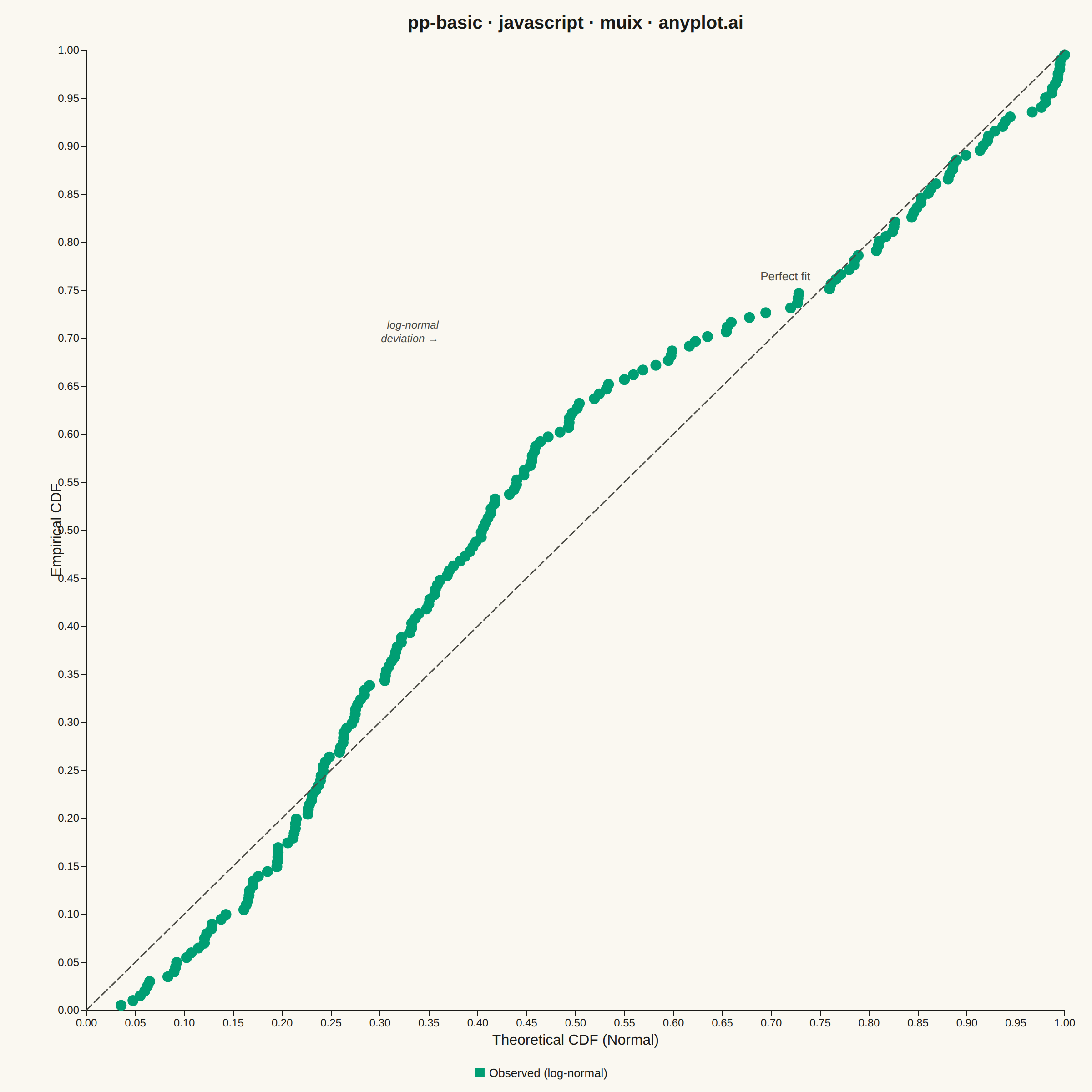
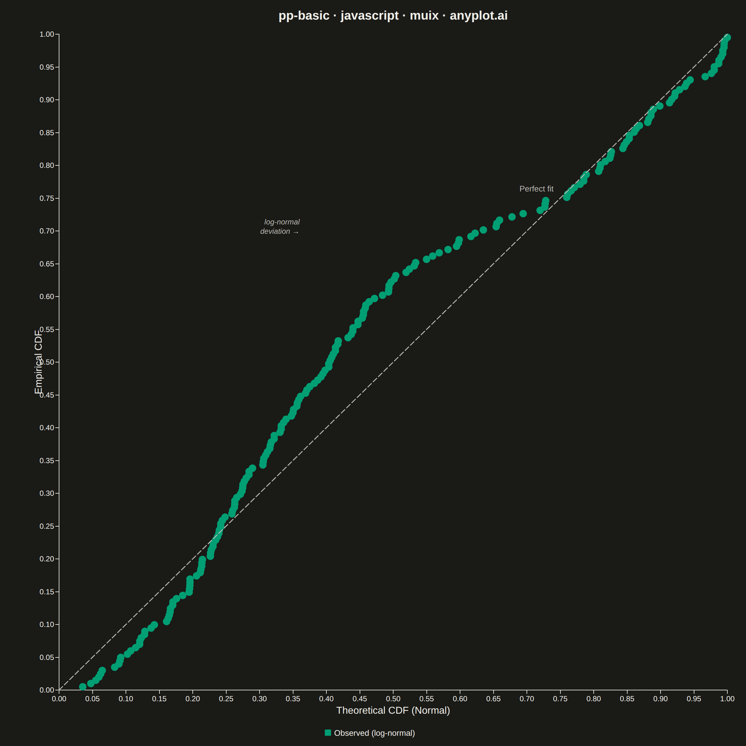
A diagnostic plot comparing the cumulative distribution function (CDF) of observed data against a theoretical distribution by plotting empirical CDF values against theoretical CDF values. Unlike Q-Q plots which compare quantiles, P-P plots compare cumulative probabilities on both axes (0 to 1), making them more sensitive to deviations in the center of the distribution. Points falling along the 45-degree diagonal indicate a good fit.
// anyplot.ai
// pp-basic: Probability-Probability (P-P) Plot
// Library: muix 7.29.1 | JavaScript 22.22.3
// Quality: 87/100 | Created: 2026-06-09
//# anyplot-orientation: square
import { ScatterChart } from "@mui/x-charts/ScatterChart";
import { useDrawingArea } from "@mui/x-charts/hooks";

const t = window.ANYPLOT_TOKENS;

// --- Utilities ---------------------------------------------------------------

function lcgRng(seed) {
  let s = seed >>> 0;
  return () => {
    s = (Math.imul(s, 1664525) + 1013904223) >>> 0;
    return s / 4294967296;
  };
}

function boxMuller(u1, u2) {
  const mag = Math.sqrt(-2 * Math.log(Math.max(u1, 1e-10)));
  return [mag * Math.cos(2 * Math.PI * u2), mag * Math.sin(2 * Math.PI * u2)];
}

// Standard normal CDF (Abramowitz & Stegun 26.2.17)
function normCDF(x) {
  const p = 0.2316419;
  const b = [0.31938153, -0.356563782, 1.781477937, -1.821255978, 1.330274429];
  const k = 1.0 / (1.0 + p * Math.abs(x));
  const poly = k * (b[0] + k * (b[1] + k * (b[2] + k * (b[3] + k * b[4]))));
  const phi = Math.exp(-0.5 * x * x) / Math.sqrt(2 * Math.PI);
  return x >= 0 ? 1.0 - phi * poly : phi * poly;
}

// --- Data (200 samples from a mildly right-skewed log-normal distribution) ---

const rng = lcgRng(42);
const samples = [];
for (let i = 0; i < 100; i++) {
  const [z0, z1] = boxMuller(rng(), rng());
  samples.push(Math.exp(0.35 * z0));
  samples.push(Math.exp(0.35 * z1));
}
samples.sort((a, b) => a - b);

const N = samples.length;
const mean = samples.reduce((s, x) => s + x, 0) / N;
const variance = samples.reduce((s, x) => s + (x - mean) ** 2, 0) / (N - 1);
const std = Math.sqrt(variance);

// Weibull plotting positions: i / (N+1), i = 1..N
const empirical = samples.map((_, i) => (i + 1) / (N + 1));
// Theoretical normal CDF with MLE-fitted mean and std
const theoretical = samples.map((x) => normCDF((x - mean) / std));

const ppData = theoretical.map((thCdf, i) => ({
  id: String(i),
  x: thCdf,
  y: empirical[i],
}));

// --- Custom SVG components ---------------------------------------------------

// 45-degree reference diagonal and annotations within the drawing area
function Overlay() {
  const { left, top, width, height } = useDrawingArea();
  return (
    <g>
      {/* 45° reference diagonal: data (0,0)→(1,1) maps to drawing-area corners */}
      <line
        x1={left}
        y1={top + height}
        x2={left + width}
        y2={top}
        stroke={t.inkSoft}
        strokeWidth={1.5}
        strokeDasharray="8 4"
        strokeLinecap="round"
      />
      {/* "Perfect fit" label — at ~78% along diagonal, clear of the upper-right data cluster */}
      <text
        x={left + width * 0.74}
        y={top + height * 0.24}
        textAnchor="end"
        fill={t.inkSoft}
        fontSize={13}
        fontFamily="-apple-system, BlinkMacSystemFont, 'Segoe UI', sans-serif"
      >
        Perfect fit
      </text>
      {/* S-curve deviation annotation near the peak separation (theoretical CDF ~0.45) */}
      <text
        x={left + width * 0.36}
        y={top + height * 0.29}
        textAnchor="end"
        fill={t.inkSoft}
        fontSize={12}
        fontStyle="italic"
        fontFamily="-apple-system, BlinkMacSystemFont, 'Segoe UI', sans-serif"
      >
        log-normal
      </text>
      <text
        x={left + width * 0.36}
        y={top + height * 0.29 + 15}
        textAnchor="end"
        fill={t.inkSoft}
        fontSize={12}
        fontStyle="italic"
        fontFamily="-apple-system, BlinkMacSystemFont, 'Segoe UI', sans-serif"
      >
        deviation →
      </text>
    </g>
  );
}

function ChartTitle() {
  const { left, width } = useDrawingArea();
  return (
    <text
      x={left + width / 2}
      y={26}
      textAnchor="middle"
      dominantBaseline="middle"
      fill={t.ink}
      fontSize={20}
      fontWeight="600"
      fontFamily="-apple-system, BlinkMacSystemFont, 'Segoe UI', sans-serif"
    >
      pp-basic · javascript · muix · anyplot.ai
    </text>
  );
}

// --- Chart -------------------------------------------------------------------

export default function Chart() {
  return (
    <ScatterChart
      width={window.ANYPLOT_SIZE.width}
      height={window.ANYPLOT_SIZE.height}
      colors={t.palette}
      skipAnimation
      margin={{ top: 55, bottom: 90, left: 95, right: 30 }}
      sx={{
        "& .MuiChartsGrid-line": { opacity: 0.15 },
      }}
      xAxis={[{
        min: 0,
        max: 1,
        label: "Theoretical CDF (Normal)",
        labelStyle: { fontSize: 16 },
        tickLabelStyle: { fontSize: 12 },
      }]}
      yAxis={[{
        min: 0,
        max: 1,
        label: "Empirical CDF",
        labelStyle: { fontSize: 16 },
        tickLabelStyle: { fontSize: 12 },
      }]}
      series={[{
        data: ppData,
        label: "Observed (log-normal)",
        markerSize: 6,
        valueFormatter: (v) =>
          `Theoretical: ${v.x.toFixed(3)}, Empirical: ${v.y.toFixed(3)}`,
      }]}
      slotProps={{
        legend: {
          position: { vertical: "bottom", horizontal: "middle" },
          itemMarkWidth: 10,
          itemMarkHeight: 10,
          labelStyle: { fontSize: 13, fontWeight: 500 },
        },
      }}
    >
      <Overlay />
      <ChartTitle />
    </ScatterChart>
  );
}
Runnable source as JSON, for any HTTP client: https://api.anyplot.ai/specs/pp-basic/muix/code. Any spec id and library id listed in llms-full.txt fit the same URL shape; every URL below is complete and callable.
{
  "spec_id": "pp-basic",
  "language": "javascript",
  "library": "muix",
  "page": "https://anyplot.ai/pp-basic/javascript/muix",
  "hub": "https://anyplot.ai/pp-basic",
  "code_json": "https://api.anyplot.ai/specs/pp-basic/muix/code",
  "spec_json": "https://api.anyplot.ai/specs/pp-basic",
  "render_light_png": "https://storage.googleapis.com/anyplot-images/plots/pp-basic/javascript/muix/plot-light.png",
  "render_dark_png": "https://storage.googleapis.com/anyplot-images/plots/pp-basic/javascript/muix/plot-dark.png",
  "interactive_light_html": "https://storage.googleapis.com/anyplot-images/plots/pp-basic/javascript/muix/plot-light.html",
  "interactive_dark_html": "https://storage.googleapis.com/anyplot-images/plots/pp-basic/javascript/muix/plot-dark.html",
  "quality_score": 87.0,
  "license": "MIT",
  "guide": "https://anyplot.ai/llms.txt"
}
Part of Probability-Probability (P-P) Plot on anyplot.ai.