The same plot in 14 other libraries — JavaScript: Chart.js, D3.js, Apache ECharts, MUI X Charts; Python: Altair, Bokeh, lets-plot, Matplotlib, Plotly, plotnine, Pygal, Seaborn; R: ggplot2; Julia: Makie.jl. Compare all 15 side by side: Probability-Probability (P-P) Plot in Python, R, Julia and JavaScript.
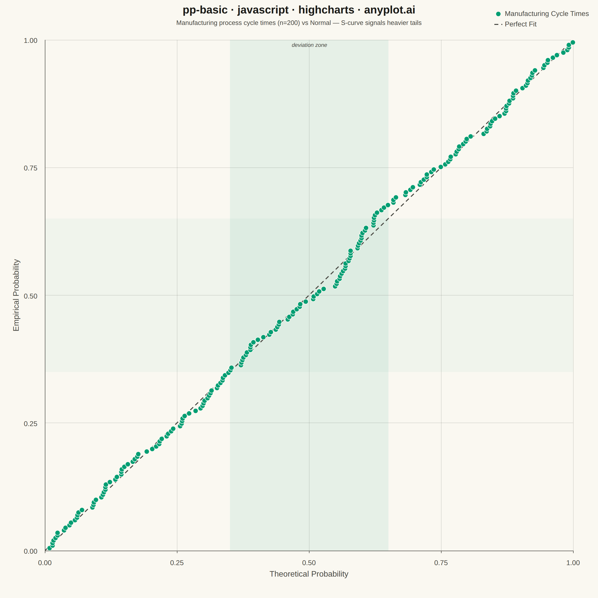
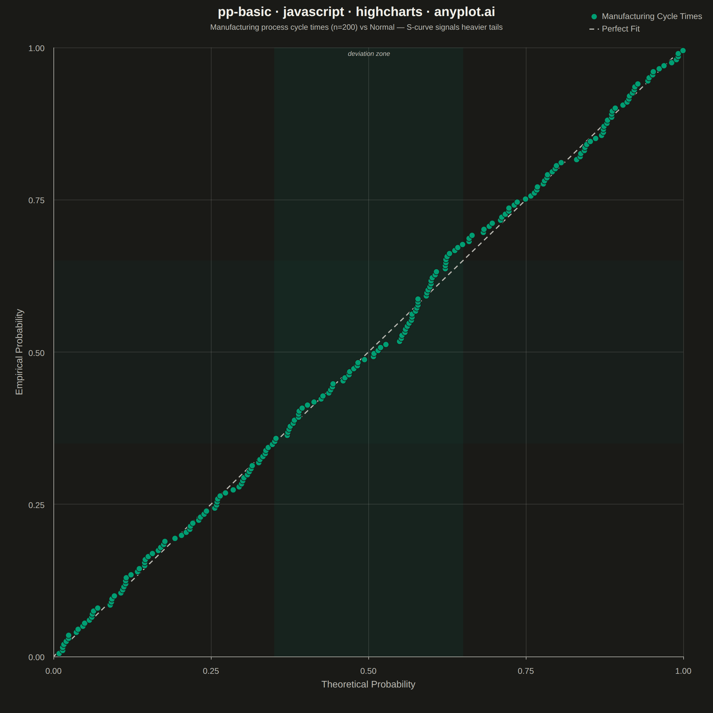
A diagnostic plot comparing the cumulative distribution function (CDF) of observed data against a theoretical distribution by plotting empirical CDF values against theoretical CDF values. Unlike Q-Q plots which compare quantiles, P-P plots compare cumulative probabilities on both axes (0 to 1), making them more sensitive to deviations in the center of the distribution. Points falling along the 45-degree diagonal indicate a good fit.
// anyplot.ai
// pp-basic: Probability-Probability (P-P) Plot
// Library: highcharts 12.6.0 | JavaScript 22.22.3
// Quality: 84/100 | Created: 2026-06-09
//# anyplot-orientation: square

const t = window.ANYPLOT_TOKENS;

// Deterministic LCG for reproducible data (no seeded RNG in browser)
let lcgState = 42;
function lcgRand() {
    lcgState = (1664525 * lcgState + 1013904223) >>> 0;
    return lcgState / 0x100000000;
}

// Box-Muller: standard normal samples
function stdNormal() {
    const u1 = Math.max(lcgRand(), 1e-10);
    const u2 = lcgRand();
    return Math.sqrt(-2 * Math.log(u1)) * Math.cos(2 * Math.PI * u2);
}

// Normal CDF via Abramowitz & Stegun rational approximation (max error ~7.5e-8)
function normalCDF(x, mu, sigma) {
    const z = (x - mu) / sigma;
    const a = Math.abs(z);
    const t0 = 1 / (1 + 0.2316419 * a);
    const poly = t0 * (0.319381530 + t0 * (-0.356563782 + t0 * (1.781477937 + t0 * (-1.821255978 + t0 * 1.330274429))));
    const phi = Math.exp(-0.5 * a * a) / Math.sqrt(2 * Math.PI);
    const p = 1 - phi * poly;
    return z >= 0 ? p : 1 - p;
}

// Generate 200 samples: right-skewed, simulating manufacturing process cycle times
// (short cycles dominate; occasional long runs create a heavier upper tail)
const N = 200;
const samples = [];
for (let i = 0; i < N; i++) {
    const base = stdNormal();
    const skew = Math.abs(stdNormal()) * 0.4;
    samples.push(base + skew);
}

// Fit normal parameters (MLE: sample mean and std)
const mean = samples.reduce((s, v) => s + v, 0) / N;
const std = Math.sqrt(samples.reduce((s, v) => s + (v - mean) ** 2, 0) / N);

// Sort and compute P-P values using plotting position i/(n+1)
const sorted = [...samples].sort((a, b) => a - b);
const ppPoints = sorted.map((x, i) => {
    const empirical = (i + 1) / (N + 1);
    const theoretical = normalCDF(x, mean, std);
    return [theoretical, empirical];
});

// 45-degree reference line (perfect distributional fit)
const refLine = [[0, 0], [1, 1]];

// Deviation zone: where the S-shaped curve crosses the diagonal (~0.35–0.65)
const devBandColor = 'rgba(0, 158, 115, 0.08)';

Highcharts.chart("container", {
    chart: {
        backgroundColor: "transparent",
        plotBorderWidth: 0,
        animation: false,
        style: { fontFamily: "inherit" },
        margin: [80, 50, 95, 90]
    },
    credits: { enabled: false },
    colors: t.palette,
    title: {
        text: "pp-basic · javascript · highcharts · anyplot.ai",
        style: { color: t.ink, fontSize: "22px", fontWeight: "600" }
    },
    subtitle: {
        text: "Manufacturing process cycle times (n=200) vs Normal — S-curve signals heavier tails",
        style: { color: t.inkSoft, fontSize: "13px" }
    },
    xAxis: {
        title: {
            text: "Theoretical Probability",
            style: { color: t.inkSoft, fontSize: "16px" }
        },
        min: 0,
        max: 1,
        tickInterval: 0.25,
        lineColor: t.inkSoft,
        lineWidth: 1,
        tickColor: t.inkSoft,
        tickLength: 5,
        gridLineColor: t.grid,
        gridLineWidth: 1,
        labels: {
            style: { color: t.inkSoft, fontSize: "14px" },
            format: "{value:.2f}"
        },
        plotBands: [{
            from: 0.35,
            to: 0.65,
            color: devBandColor,
            zIndex: 0,
            label: {
                text: "deviation zone",
                align: "center",
                verticalAlign: "top",
                y: 14,
                style: { color: t.inkSoft, fontSize: "11px", fontStyle: "italic" }
            }
        }]
    },
    yAxis: {
        title: {
            text: "Empirical Probability",
            style: { color: t.inkSoft, fontSize: "16px" }
        },
        min: 0,
        max: 1,
        tickInterval: 0.25,
        lineColor: t.inkSoft,
        lineWidth: 1,
        tickColor: t.inkSoft,
        tickLength: 5,
        gridLineColor: t.grid,
        gridLineWidth: 1,
        labels: {
            style: { color: t.inkSoft, fontSize: "14px" },
            format: "{value:.2f}"
        },
        plotBands: [{
            from: 0.35,
            to: 0.65,
            color: "rgba(0, 158, 115, 0.04)",
            zIndex: 0
        }]
    },
    legend: {
        enabled: true,
        align: "right",
        verticalAlign: "top",
        layout: "vertical",
        itemStyle: { color: t.inkSoft, fontSize: "14px" },
        itemHoverStyle: { color: t.ink }
    },
    tooltip: { enabled: false },
    plotOptions: {
        series: { animation: false },
        scatter: {
            marker: {
                radius: 5,
                symbol: "circle",
                lineWidth: 1,
                lineColor: t.pageBg
            }
        }
    },
    series: [
        {
            type: "scatter",
            name: "Manufacturing Cycle Times",
            data: ppPoints,
            color: t.palette[0],
            zIndex: 2
        },
        {
            type: "line",
            name: "Perfect Fit",
            data: refLine,
            color: t.inkSoft,
            dashStyle: "Dash",
            lineWidth: 2,
            marker: { enabled: false },
            enableMouseTracking: false,
            zIndex: 1
        }
    ]
});
Runnable source as JSON, for any HTTP client: https://api.anyplot.ai/specs/pp-basic/highcharts/code. Any spec id and library id listed in llms-full.txt fit the same URL shape; every URL below is complete and callable.
{
  "spec_id": "pp-basic",
  "language": "javascript",
  "library": "highcharts",
  "page": "https://anyplot.ai/pp-basic/javascript/highcharts",
  "hub": "https://anyplot.ai/pp-basic",
  "code_json": "https://api.anyplot.ai/specs/pp-basic/highcharts/code",
  "spec_json": "https://api.anyplot.ai/specs/pp-basic",
  "render_light_png": "https://storage.googleapis.com/anyplot-images/plots/pp-basic/javascript/highcharts/plot-light.png",
  "render_dark_png": "https://storage.googleapis.com/anyplot-images/plots/pp-basic/javascript/highcharts/plot-dark.png",
  "interactive_light_html": "https://storage.googleapis.com/anyplot-images/plots/pp-basic/javascript/highcharts/plot-light.html",
  "interactive_dark_html": "https://storage.googleapis.com/anyplot-images/plots/pp-basic/javascript/highcharts/plot-dark.html",
  "quality_score": 84.0,
  "license": "MIT",
  "guide": "https://anyplot.ai/llms.txt"
}
Part of Probability-Probability (P-P) Plot on anyplot.ai.