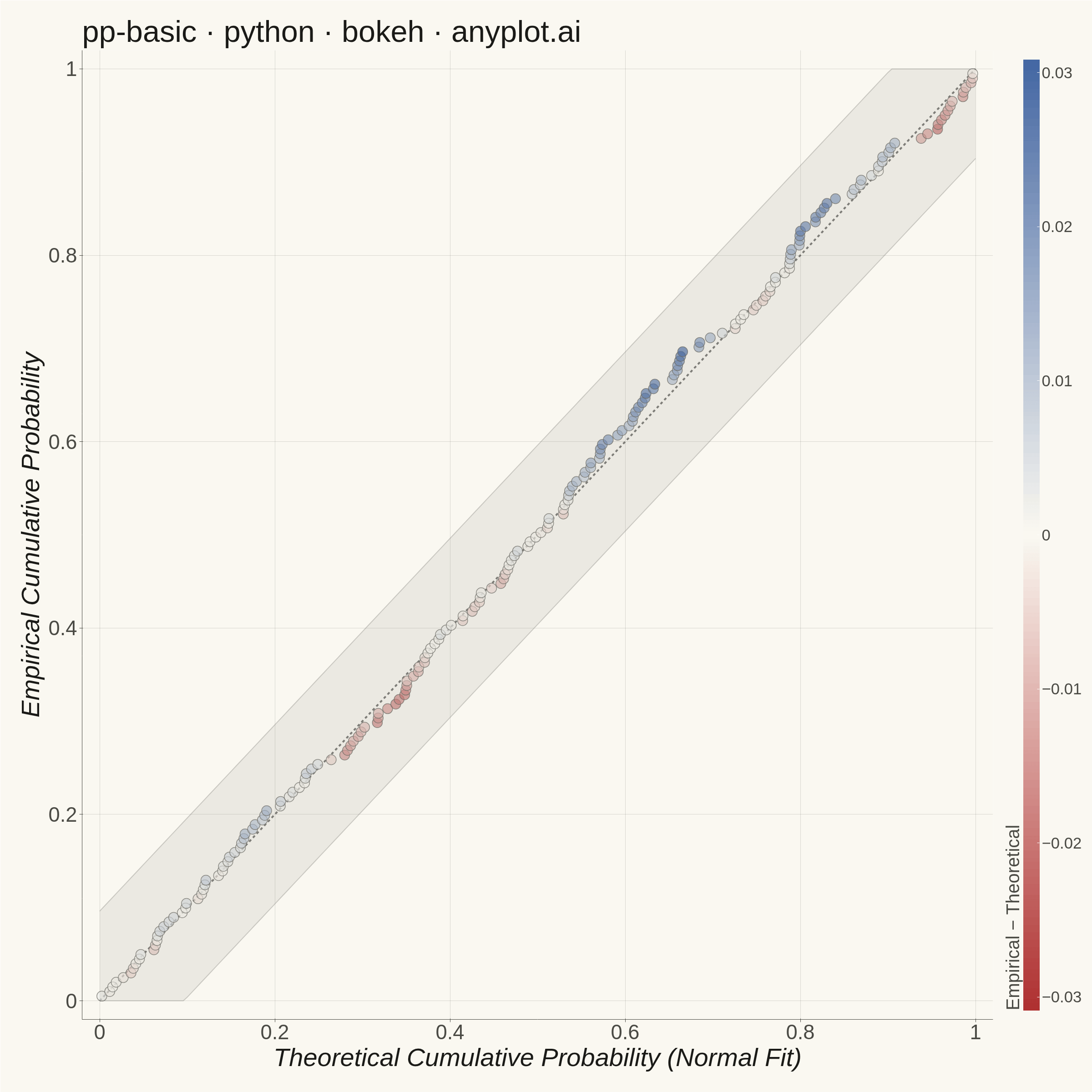
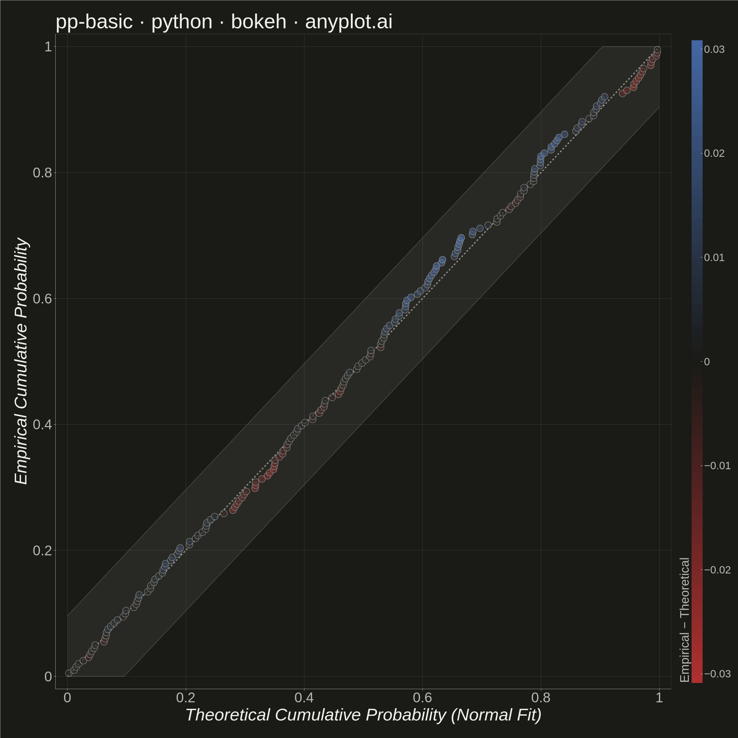
A diagnostic plot comparing the cumulative distribution function (CDF) of observed data against a theoretical distribution by plotting empirical CDF values against theoretical CDF values. Unlike Q-Q plots which compare quantiles, P-P plots compare cumulative probabilities on both axes (0 to 1), making them more sensitive to deviations in the center of the distribution. Points falling along the 45-degree diagonal indicate a good fit.
""" anyplot.ai
pp-basic: Probability-Probability (P-P) Plot
Library: bokeh 3.9.1 | Python 3.13.13
Quality: 93/100 | Updated: 2026-06-16
"""

import io
import os
import time
from pathlib import Path

import numpy as np
from bokeh.io import output_file, save
from bokeh.models import Band, ColorBar, ColumnDataSource, HoverTool, LinearColorMapper
from bokeh.plotting import figure
from bokeh.transform import transform
from PIL import Image
from scipy import stats
from selenium import webdriver
from selenium.webdriver.chrome.options import Options


# Theme tokens (see prompts/default-style-guide.md "Theme-adaptive Chrome")
THEME = os.getenv("ANYPLOT_THEME", "light")
PAGE_BG = "#FAF8F1" if THEME == "light" else "#1A1A17"
INK = "#1A1A17" if THEME == "light" else "#F0EFE8"
INK_SOFT = "#4A4A44" if THEME == "light" else "#B8B7B0"
MUTED = "#6B6A63" if THEME == "light" else "#A8A79F"

# Imprint diverging colormap — matte-red <-> theme midpoint <-> blue (signed deviation)
mid_hex = "#FAF8F1" if THEME == "light" else "#1A1A17"
red_rgb = np.array([0xAE, 0x30, 0x30])
blue_rgb = np.array([0x44, 0x67, 0xA3])
mid_rgb = np.array([int(mid_hex[i : i + 2], 16) for i in (1, 3, 5)])
ramp_t = np.linspace(0, 1, 128)[:, None]
div_rgb = np.vstack([red_rgb * (1 - ramp_t) + mid_rgb * ramp_t, mid_rgb * (1 - ramp_t) + blue_rgb * ramp_t])
IMPRINT_DIV256 = ["#%02X%02X%02X" % tuple(c) for c in div_rgb.round().astype(int)]

# Data — manufacturing QC: bolt tensile strength (right-skewed vs. normal reference)
np.random.seed(42)
bolt_strength = np.random.normal(loc=850, scale=45, size=200) + np.random.exponential(scale=15, size=200)
observed_sorted = np.sort(bolt_strength)
n = len(observed_sorted)

mu, sigma = stats.norm.fit(observed_sorted)
empirical_cdf = np.arange(1, n + 1) / (n + 1)
theoretical_cdf = stats.norm.cdf(observed_sorted, loc=mu, scale=sigma)
deviation = empirical_cdf - theoretical_cdf

# Kolmogorov-Smirnov 95% confidence band, clipped to [0, 1]
ks_bound = 1.36 / np.sqrt(n)
band_x = np.linspace(0, 1, 200)
band_source = ColumnDataSource(
    data={"x": band_x, "upper": np.clip(band_x + ks_bound, 0, 1), "lower": np.clip(band_x - ks_bound, 0, 1)}
)

source = ColumnDataSource(
    data={
        "theoretical": theoretical_cdf,
        "empirical": empirical_cdf,
        "deviation": deviation,
        "strength": observed_sorted,
        "rank": np.arange(1, n + 1),
    }
)

max_dev = float(np.max(np.abs(deviation)))
color_mapper = LinearColorMapper(palette=IMPRINT_DIV256, low=-max_dev, high=max_dev)

# Plot — square canvas preserves the diagonal's visual meaning
p = figure(
    width=2400,
    height=2400,
    title="pp-basic · python · bokeh · anyplot.ai",
    x_axis_label="Theoretical Cumulative Probability (Normal Fit)",
    y_axis_label="Empirical Cumulative Probability",
    x_range=(-0.02, 1.02),
    y_range=(-0.02, 1.02),
    toolbar_location=None,
    min_border_bottom=160,
    min_border_left=180,
    min_border_top=110,
    min_border_right=60,
)

# KS confidence band (muted structural layer, sits behind the data)
band = Band(
    base="x",
    upper="upper",
    lower="lower",
    source=band_source,
    fill_alpha=0.10,
    fill_color=MUTED,
    line_color=MUTED,
    line_alpha=0.3,
    line_width=2,
)
p.add_layout(band)

# 45-degree reference line — perfect-fit baseline (neutral anchor)
p.line([0, 1], [0, 1], line_color=INK, line_width=4, line_dash="dashed", line_alpha=0.55)

# Data points colored by signed deviation from the diagonal
scatter = p.scatter(
    x="theoretical",
    y="empirical",
    source=source,
    size=22,
    fill_color=transform("deviation", color_mapper),
    fill_alpha=0.65,
    line_color=MUTED,  # soft ink ring keeps near-zero-deviation points legible
    line_alpha=0.7,
    line_width=1.5,
)

# HoverTool — Bokeh-distinctive interactive inspection
hover = HoverTool(
    renderers=[scatter],
    tooltips=[
        ("Bolt Strength", "@strength{0.1} MPa"),
        ("Rank", "@rank / 200"),
        ("Theoretical P", "@theoretical{0.000}"),
        ("Empirical P", "@empirical{0.000}"),
        ("Deviation", "@deviation{+0.000}"),
    ],
    mode="mouse",
)
p.add_tools(hover)

# Colorbar legend for the continuous deviation encoding
color_bar = ColorBar(
    color_mapper=color_mapper,
    title="Empirical − Theoretical",
    title_text_font_size="30pt",
    title_text_color=INK_SOFT,
    title_text_font_style="normal",
    major_label_text_font_size="26pt",
    major_label_text_color=INK_SOFT,
    background_fill_color=PAGE_BG,
    width=36,
    padding=20,
    bar_line_color=None,
)
p.add_layout(color_bar, "right")

# Style — theme-adaptive chrome
p.title.text_font_size = "50pt"
p.title.text_font_style = "normal"
p.title.text_color = INK
p.xaxis.axis_label_text_font_size = "42pt"
p.yaxis.axis_label_text_font_size = "42pt"
p.xaxis.major_label_text_font_size = "34pt"
p.yaxis.major_label_text_font_size = "34pt"
p.xaxis.axis_label_text_color = INK
p.yaxis.axis_label_text_color = INK
p.xaxis.major_label_text_color = INK_SOFT
p.yaxis.major_label_text_color = INK_SOFT

p.xaxis.minor_tick_line_color = None
p.yaxis.minor_tick_line_color = None
p.xaxis.major_tick_line_color = INK_SOFT
p.yaxis.major_tick_line_color = INK_SOFT
p.xaxis.axis_line_color = INK_SOFT
p.yaxis.axis_line_color = INK_SOFT
p.xaxis[0].ticker.desired_num_ticks = 6
p.yaxis[0].ticker.desired_num_ticks = 6

p.xgrid.grid_line_color = INK
p.ygrid.grid_line_color = INK
p.xgrid.grid_line_alpha = 0.15
p.ygrid.grid_line_alpha = 0.15

p.outline_line_color = None
p.background_fill_color = PAGE_BG
p.border_fill_color = PAGE_BG

# Save — interactive HTML, then screenshot it with headless Chrome
output_file(f"plot-{THEME}.html", title="pp-basic · python · bokeh · anyplot.ai")
save(p)

# Window is taller than the canvas so bokeh fills it; crop to the exact dims.
W, H = 2400, 2400
opts = Options()
for arg in (
    "--headless=new",
    "--no-sandbox",
    "--disable-dev-shm-usage",
    "--disable-gpu",
    f"--window-size={W},{H + 200}",
    "--hide-scrollbars",
):
    opts.add_argument(arg)
driver = webdriver.Chrome(options=opts)
driver.set_window_size(W, H + 200)
driver.get(f"file://{Path(f'plot-{THEME}.html').resolve()}")
time.sleep(3)
raw = driver.get_screenshot_as_png()
driver.quit()
Image.open(io.BytesIO(raw)).crop((0, 0, W, H)).save(f"plot-{THEME}.png")
Runnable source as JSON, for any HTTP client: https://api.anyplot.ai/specs/pp-basic/bokeh/code. Any spec id and library id listed in llms-full.txt fit the same URL shape; every URL below is complete and callable.
{
  "spec_id": "pp-basic",
  "language": "python",
  "library": "bokeh",
  "page": "https://anyplot.ai/pp-basic/python/bokeh",
  "hub": "https://anyplot.ai/pp-basic",
  "code_json": "https://api.anyplot.ai/specs/pp-basic/bokeh/code",
  "spec_json": "https://api.anyplot.ai/specs/pp-basic",
  "render_light_png": "https://storage.googleapis.com/anyplot-images/plots/pp-basic/python/bokeh/plot-light.png",
  "render_dark_png": "https://storage.googleapis.com/anyplot-images/plots/pp-basic/python/bokeh/plot-dark.png",
  "interactive_light_html": "https://storage.googleapis.com/anyplot-images/plots/pp-basic/python/bokeh/plot-light.html",
  "interactive_dark_html": "https://storage.googleapis.com/anyplot-images/plots/pp-basic/python/bokeh/plot-dark.html",
  "quality_score": 93.0,
  "license": "MIT",
  "guide": "https://anyplot.ai/llms.txt"
}
Part of Probability-Probability (P-P) Plot on anyplot.ai.