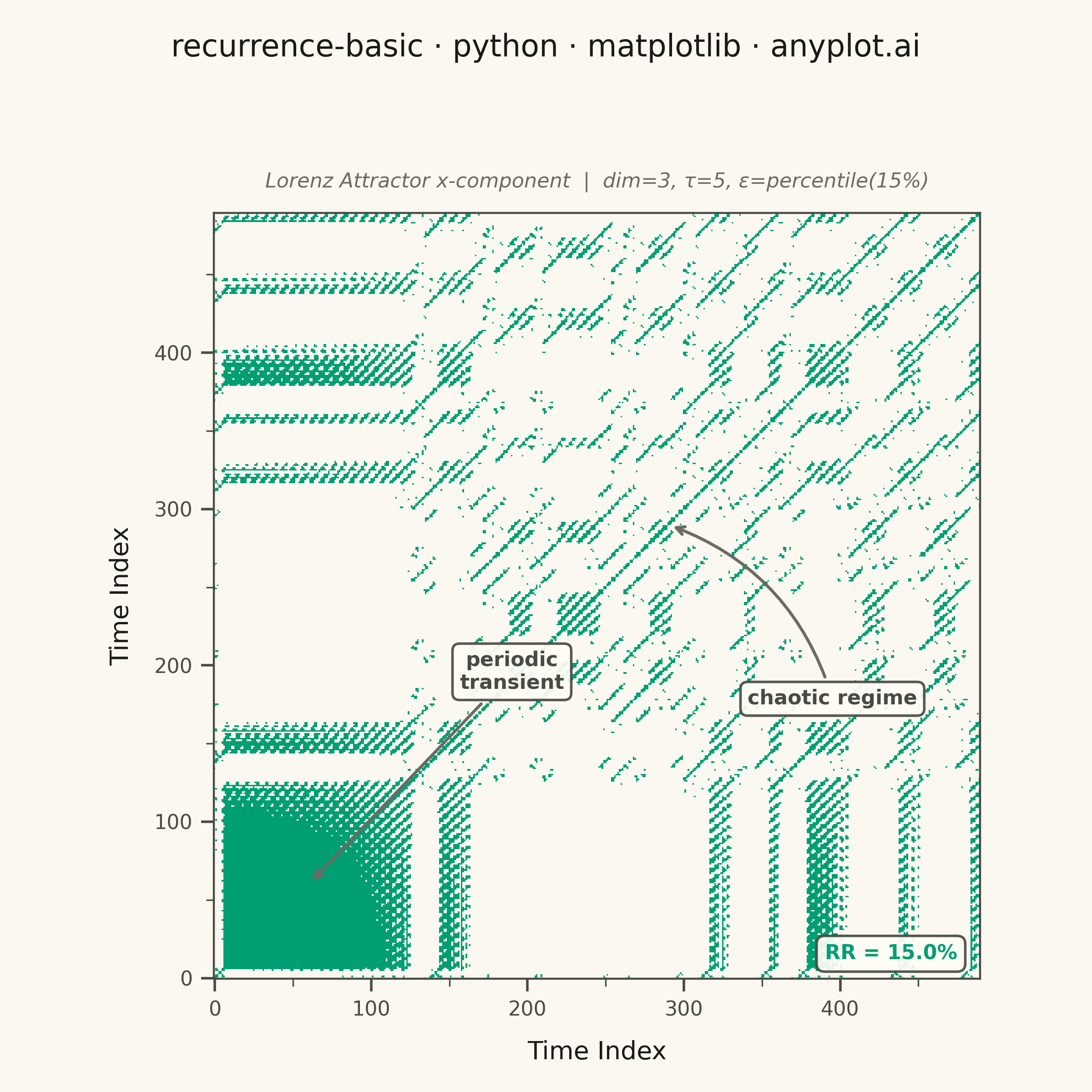
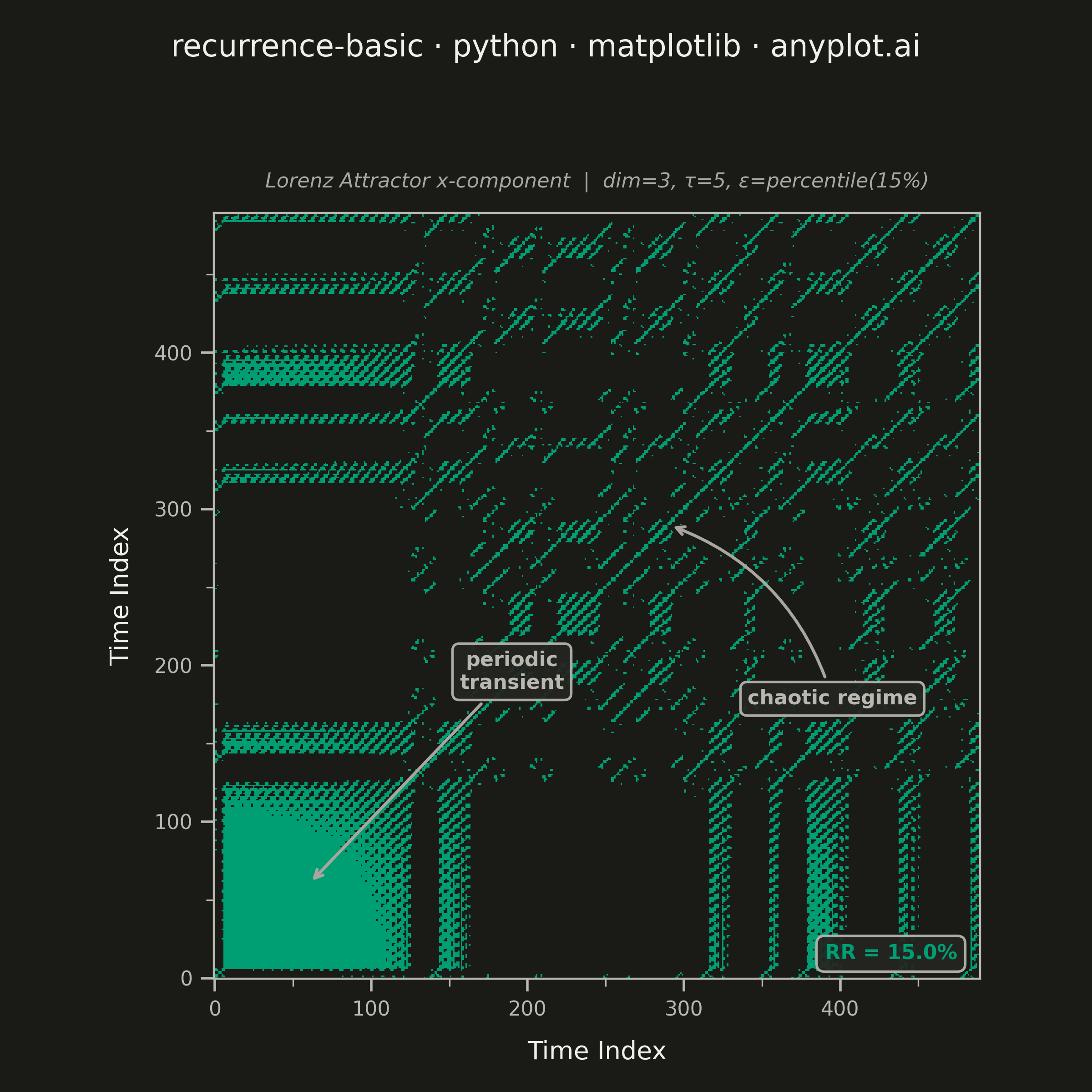
A recurrence plot is a binary or distance-based matrix visualization that reveals when states in a dynamical system recur over time. Both axes represent time indices, and a point is plotted at position (i, j) when the system state at time i is sufficiently similar to the state at time j (distance below a threshold). The resulting symmetric matrix exposes hidden structure in complex, nonlinear dynamics — diagonal lines indicate determinism, vertical/horizontal lines reveal laminar states, and block structures signal regime changes.
""" anyplot.ai
recurrence-basic: Recurrence Plot for Nonlinear Time Series
Library: matplotlib 3.10.9 | Python 3.13.13
Quality: 90/100 | Updated: 2026-06-10
"""

import os

import matplotlib.pyplot as plt
import matplotlib.ticker as ticker
import numpy as np
from matplotlib.colors import BoundaryNorm, ListedColormap
from scipy.integrate import solve_ivp
from scipy.spatial.distance import cdist


# Theme tokens (Imprint palette — see prompts/default-style-guide.md)
THEME = os.getenv("ANYPLOT_THEME", "light")
PAGE_BG = "#FAF8F1" if THEME == "light" else "#1A1A17"
ELEVATED_BG = "#FFFDF6" if THEME == "light" else "#242420"
INK = "#1A1A17" if THEME == "light" else "#F0EFE8"
INK_SOFT = "#4A4A44" if THEME == "light" else "#B8B7B0"
INK_MUTED = "#6B6A63" if THEME == "light" else "#A8A79F"
BRAND = "#009E73"  # Imprint palette position 1 — always first series

# Data — Lorenz attractor x-component via ODE solver
sol = solve_ivp(
    lambda t, s: [10.0 * (s[1] - s[0]), s[0] * (28.0 - s[2]) - s[1], s[0] * s[1] - (8.0 / 3.0) * s[2]],
    [0, 50],
    [1.0, 1.0, 1.0],
    t_eval=np.linspace(0, 50, 5000),
    max_step=0.01,
)
signal = sol.y[0][::10]  # 500 points from x-component

# Time-delay embedding (Takens' theorem: dim=3, delay=5)
embedding_dim = 3
delay = 5
n_embedded = len(signal) - (embedding_dim - 1) * delay
embedded = np.column_stack([signal[i * delay : i * delay + n_embedded] for i in range(embedding_dim)])

# Euclidean distance matrix and binary threshold
distance_matrix = cdist(embedded, embedded, metric="euclidean")
threshold = np.percentile(distance_matrix, 15)
recurrence_matrix = (distance_matrix <= threshold).astype(int)

# Plot — square canvas for symmetric matrix (2400×2400 px)
fig, ax = plt.subplots(figsize=(6, 6), dpi=400, facecolor=PAGE_BG)
ax.set_facecolor(PAGE_BG)

# Binary colormap: PAGE_BG for non-recurrent, Imprint brand green for recurrent
cmap = ListedColormap([PAGE_BG, BRAND])
norm = BoundaryNorm([0, 0.5, 1], cmap.N)
ax.imshow(recurrence_matrix, cmap=cmap, norm=norm, origin="lower", interpolation="none", aspect="equal")

# Axis labels and ticks
ax.set_xlabel("Time Index", fontsize=10, color=INK, labelpad=8)
ax.set_ylabel("Time Index", fontsize=10, color=INK, labelpad=8)
ax.xaxis.set_major_locator(ticker.MultipleLocator(100))
ax.yaxis.set_major_locator(ticker.MultipleLocator(100))
ax.xaxis.set_minor_locator(ticker.MultipleLocator(50))
ax.yaxis.set_minor_locator(ticker.MultipleLocator(50))
ax.xaxis.set_major_formatter(ticker.FuncFormatter(lambda x, _: f"{int(x)}"))
ax.yaxis.set_major_formatter(ticker.FuncFormatter(lambda x, _: f"{int(x)}"))
ax.tick_params(axis="both", which="major", labelsize=8, length=5, width=1.0, colors=INK_SOFT)
ax.tick_params(axis="both", which="minor", length=3, width=0.6, colors=INK_SOFT)

for spine in ax.spines.values():
    spine.set_color(INK_SOFT)
    spine.set_linewidth(0.8)

# Regime annotations — elevated background boxes ensure text is always readable
ax.annotate(
    "periodic\ntransient",
    xy=(60, 60),
    xytext=(190, 185),
    fontsize=8,
    color=INK_SOFT,
    fontweight="bold",
    ha="center",
    arrowprops={"arrowstyle": "->", "color": INK_MUTED, "lw": 1.2},
    bbox={"facecolor": ELEVATED_BG, "edgecolor": INK_SOFT, "alpha": 0.92, "boxstyle": "round,pad=0.45"},
)
ax.annotate(
    "chaotic regime",
    xy=(290, 290),
    xytext=(395, 175),
    fontsize=8,
    color=INK_SOFT,
    fontweight="bold",
    ha="center",
    arrowprops={"arrowstyle": "->", "color": INK_MUTED, "lw": 1.2, "connectionstyle": "arc3,rad=0.25"},
    bbox={"facecolor": ELEVATED_BG, "edgecolor": INK_SOFT, "alpha": 0.92, "boxstyle": "round,pad=0.45"},
)

rr = np.sum(recurrence_matrix) / recurrence_matrix.size * 100
ax.text(
    0.97,
    0.02,
    f"RR = {rr:.1f}%",
    transform=ax.transAxes,
    fontsize=8,
    ha="right",
    va="bottom",
    bbox={"boxstyle": "round,pad=0.4", "facecolor": ELEVATED_BG, "edgecolor": INK_SOFT, "alpha": 0.92},
    color=BRAND,
    fontweight="bold",
)

# Titles — suptitle for mandatory format, subtitle for embedding context
fig.suptitle("recurrence-basic · python · matplotlib · anyplot.ai", fontsize=12, fontweight="medium", color=INK, y=0.97)
ax.set_title(
    "Lorenz Attractor x-component  |  dim=3, τ=5, ε=percentile(15%)",
    fontsize=9,
    color=INK_MUTED,
    style="italic",
    pad=10,
)

# Save — figsize=(6,6) dpi=400 → exact 2400×2400 px; no bbox_inches='tight'
plt.tight_layout(rect=[0.02, 0.02, 0.98, 0.92])
plt.savefig(f"plot-{THEME}.png", dpi=400, facecolor=PAGE_BG)
Runnable source as JSON, for any HTTP client: https://api.anyplot.ai/specs/recurrence-basic/matplotlib/code. Any spec id and library id listed in llms-full.txt fit the same URL shape; every URL below is complete and callable.
{
  "spec_id": "recurrence-basic",
  "language": "python",
  "library": "matplotlib",
  "page": "https://anyplot.ai/recurrence-basic/python/matplotlib",
  "hub": "https://anyplot.ai/recurrence-basic",
  "code_json": "https://api.anyplot.ai/specs/recurrence-basic/matplotlib/code",
  "spec_json": "https://api.anyplot.ai/specs/recurrence-basic",
  "render_light_png": "https://storage.googleapis.com/anyplot-images/plots/recurrence-basic/python/matplotlib/plot-light.png",
  "render_dark_png": "https://storage.googleapis.com/anyplot-images/plots/recurrence-basic/python/matplotlib/plot-dark.png",
  "quality_score": 90.0,
  "license": "MIT",
  "guide": "https://anyplot.ai/llms.txt"
}
Part of Recurrence Plot for Nonlinear Time Series on anyplot.ai.