The same plot in 14 other libraries — Python: Altair, Bokeh, lets-plot, Matplotlib, Plotly, plotnine, Pygal, Seaborn; Julia: Makie.jl; JavaScript: Chart.js, D3.js, Apache ECharts, Highcharts, MUI X Charts. Compare all 15 side by side: Recurrence Plot for Nonlinear Time Series in Python, R, Julia and JavaScript.
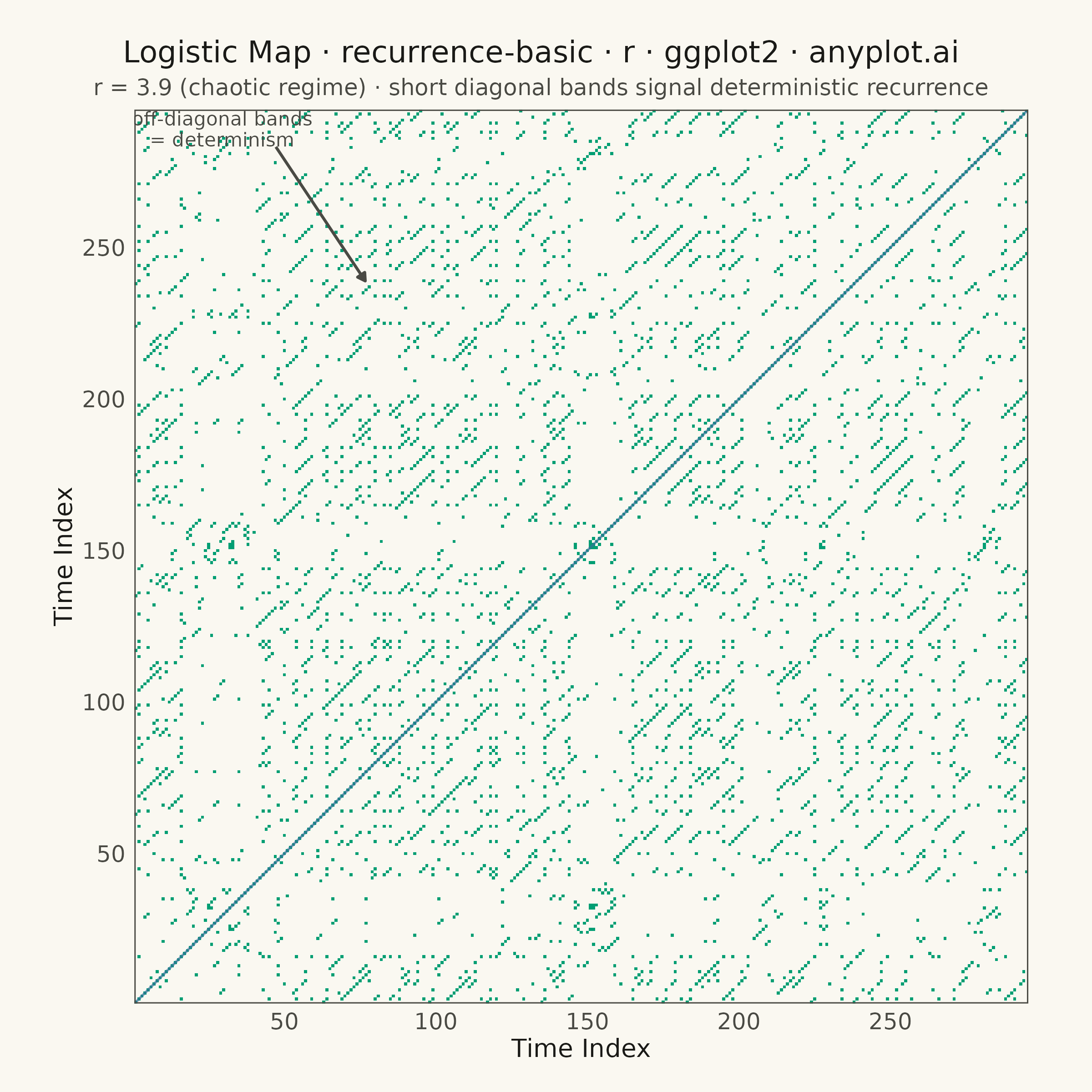
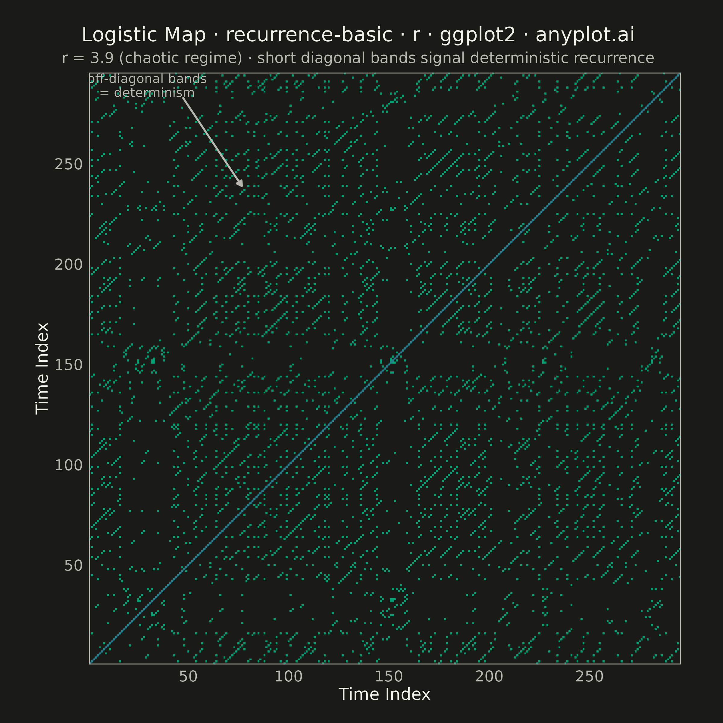
A recurrence plot is a binary or distance-based matrix visualization that reveals when states in a dynamical system recur over time. Both axes represent time indices, and a point is plotted at position (i, j) when the system state at time i is sufficiently similar to the state at time j (distance below a threshold). The resulting symmetric matrix exposes hidden structure in complex, nonlinear dynamics — diagonal lines indicate determinism, vertical/horizontal lines reveal laminar states, and block structures signal regime changes.
#' anyplot.ai
#' recurrence-basic: Recurrence Plot for Nonlinear Time Series
#' Library: ggplot2 3.5.1 | R 4.4.1
#' Quality: 88/100 | Created: 2026-06-10

library(ggplot2)
library(ragg)

set.seed(42)

# Theme tokens — Imprint palette, theme-adaptive chrome
THEME       <- Sys.getenv("ANYPLOT_THEME", "light")
PAGE_BG     <- if (THEME == "light") "#FAF8F1" else "#1A1A17"
ELEVATED_BG <- if (THEME == "light") "#FFFDF6" else "#242420"
INK         <- if (THEME == "light") "#1A1A17" else "#F0EFE8"
INK_SOFT    <- if (THEME == "light") "#4A4A44" else "#B8B7B0"
IMPRINT_PALETTE <- c(
  "#009E73",  # 1 — brand green (first categorical series)
  "#C475FD",  # 2 — lavender
  "#4467A3",  # 3 — blue
  "#BD8233",  # 4 — ochre
  "#AE3030",  # 5 — matte red
  "#2ABCCD",  # 6 — cyan
  "#954477",  # 7 — rose
  "#99B314"   # 8 — lime
)

# Data: logistic map in chaotic regime (r = 3.9, 300 steps)
n_steps <- 300
r_param <- 3.9
x_series <- numeric(n_steps)
x_series[1] <- 0.4
for (i in 2:n_steps) {
  x_series[i] <- r_param * x_series[i - 1] * (1 - x_series[i - 1])
}

# Time-delay embedding (Takens' theorem): dim = 2, delay = 5
emb_dim <- 2
delay   <- 5
n_emb   <- n_steps - (emb_dim - 1) * delay
states  <- matrix(0.0, nrow = n_emb, ncol = emb_dim)
for (d in seq_len(emb_dim)) {
  start_idx  <- (d - 1) * delay + 1
  states[, d] <- x_series[start_idx:(start_idx + n_emb - 1)]
}

# Pairwise Euclidean distances; binary threshold at 5th percentile
dist_mat      <- as.matrix(dist(states))
nonzero_dists <- dist_mat[dist_mat > 0]
epsilon       <- quantile(nonzero_dists, 0.05)
recurrence    <- as.integer(dist_mat <= epsilon)

# Long data frame for geom_raster
n_pts  <- nrow(states)
rec_df <- data.frame(
  i         = rep(seq_len(n_pts), times = n_pts),
  j         = rep(seq_len(n_pts), each  = n_pts),
  recurrent = recurrence
)

plot_title    <- "Logistic Map · recurrence-basic · r · ggplot2 · anyplot.ai"
plot_subtitle <- "r = 3.9 (chaotic regime) · short diagonal bands signal deterministic recurrence"

# Plot: binary recurrence matrix with diagonal reference + storytelling annotation
p <- ggplot(rec_df, aes(x = i, y = j, fill = factor(recurrent))) +
  geom_raster(interpolate = FALSE) +
  # Diagonal reference line emphasising the main recurrence axis (LOI)
  geom_abline(
    slope = 1, intercept = 0,
    color = IMPRINT_PALETTE[3], linewidth = 0.5, alpha = 0.55
  ) +
  # Arrow annotation pointing to off-diagonal band structure
  annotate(
    "segment",
    x = n_pts * 0.16, xend = n_pts * 0.26,
    y = n_pts * 0.96, yend = n_pts * 0.81,
    arrow = arrow(length = unit(0.12, "cm"), type = "closed"),
    color = INK_SOFT, linewidth = 0.55
  ) +
  annotate(
    "text",
    x = n_pts * 0.10, y = n_pts * 0.98,
    label = "off-diagonal bands\n= determinism",
    color = INK_SOFT, size = 2.7, hjust = 0.5, lineheight = 0.9
  ) +
  scale_fill_manual(
    values = c("0" = PAGE_BG, "1" = IMPRINT_PALETTE[1]),
    guide  = "none"
  ) +
  scale_x_continuous(expand = c(0, 0), breaks = seq(50, n_pts, by = 50)) +
  scale_y_continuous(expand = c(0, 0), breaks = seq(50, n_pts, by = 50)) +
  coord_fixed(ratio = 1) +
  labs(
    title    = plot_title,
    subtitle = plot_subtitle,
    x        = "Time Index",
    y        = "Time Index"
  ) +
  theme_minimal(base_size = 8) +
  theme(
    plot.background     = element_rect(fill = PAGE_BG, color = PAGE_BG),
    panel.background    = element_rect(fill = PAGE_BG, color = NA),
    panel.grid.major    = element_blank(),
    panel.grid.minor    = element_blank(),
    panel.border        = element_rect(color = INK_SOFT, fill = NA, linewidth = 0.5),
    axis.title          = element_text(color = INK,      size = 10),
    axis.text           = element_text(color = INK_SOFT, size = 9),
    plot.title          = element_text(color = INK,      size = 12, hjust = 0.5),
    plot.subtitle       = element_text(color = INK_SOFT, size = 9,  hjust = 0.5),
    plot.title.position = "plot",
    plot.margin         = margin(16, 16, 12, 12, unit = "pt")
  )

# Save — square canvas: 2400 × 2400 px (width=6, height=6, dpi=400)
ggsave(
  filename = sprintf("plot-%s.png", THEME),
  plot     = p,
  device   = ragg::agg_png,
  width    = 6,
  height   = 6,
  units    = "in",
  dpi      = 400
)
Runnable source as JSON, for any HTTP client: https://api.anyplot.ai/specs/recurrence-basic/ggplot2/code. Any spec id and library id listed in llms-full.txt fit the same URL shape; every URL below is complete and callable.
{
  "spec_id": "recurrence-basic",
  "language": "r",
  "library": "ggplot2",
  "page": "https://anyplot.ai/recurrence-basic/r/ggplot2",
  "hub": "https://anyplot.ai/recurrence-basic",
  "code_json": "https://api.anyplot.ai/specs/recurrence-basic/ggplot2/code",
  "spec_json": "https://api.anyplot.ai/specs/recurrence-basic",
  "render_light_png": "https://storage.googleapis.com/anyplot-images/plots/recurrence-basic/r/ggplot2/plot-light.png",
  "render_dark_png": "https://storage.googleapis.com/anyplot-images/plots/recurrence-basic/r/ggplot2/plot-dark.png",
  "quality_score": 88.0,
  "license": "MIT",
  "guide": "https://anyplot.ai/llms.txt"
}
Part of Recurrence Plot for Nonlinear Time Series on anyplot.ai.