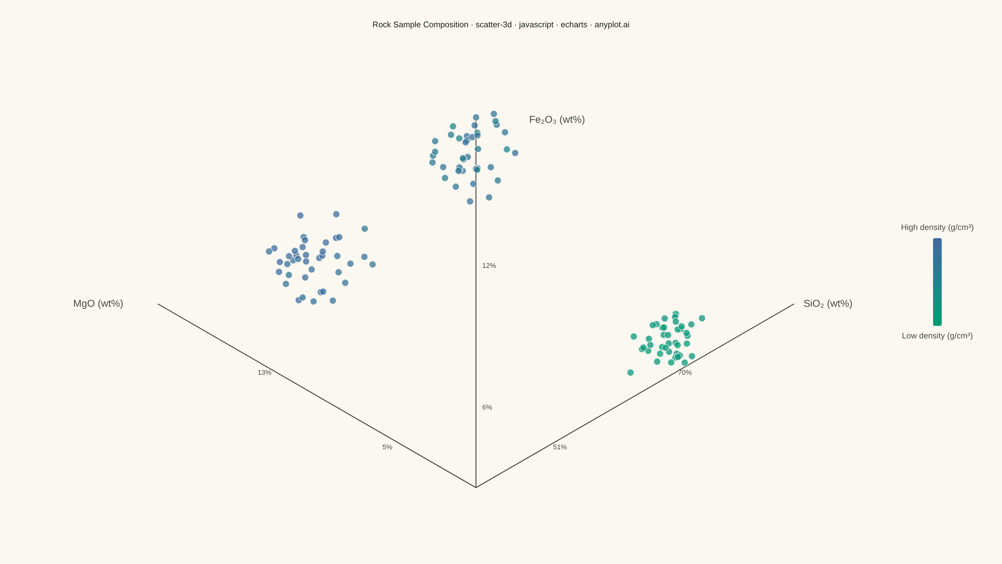
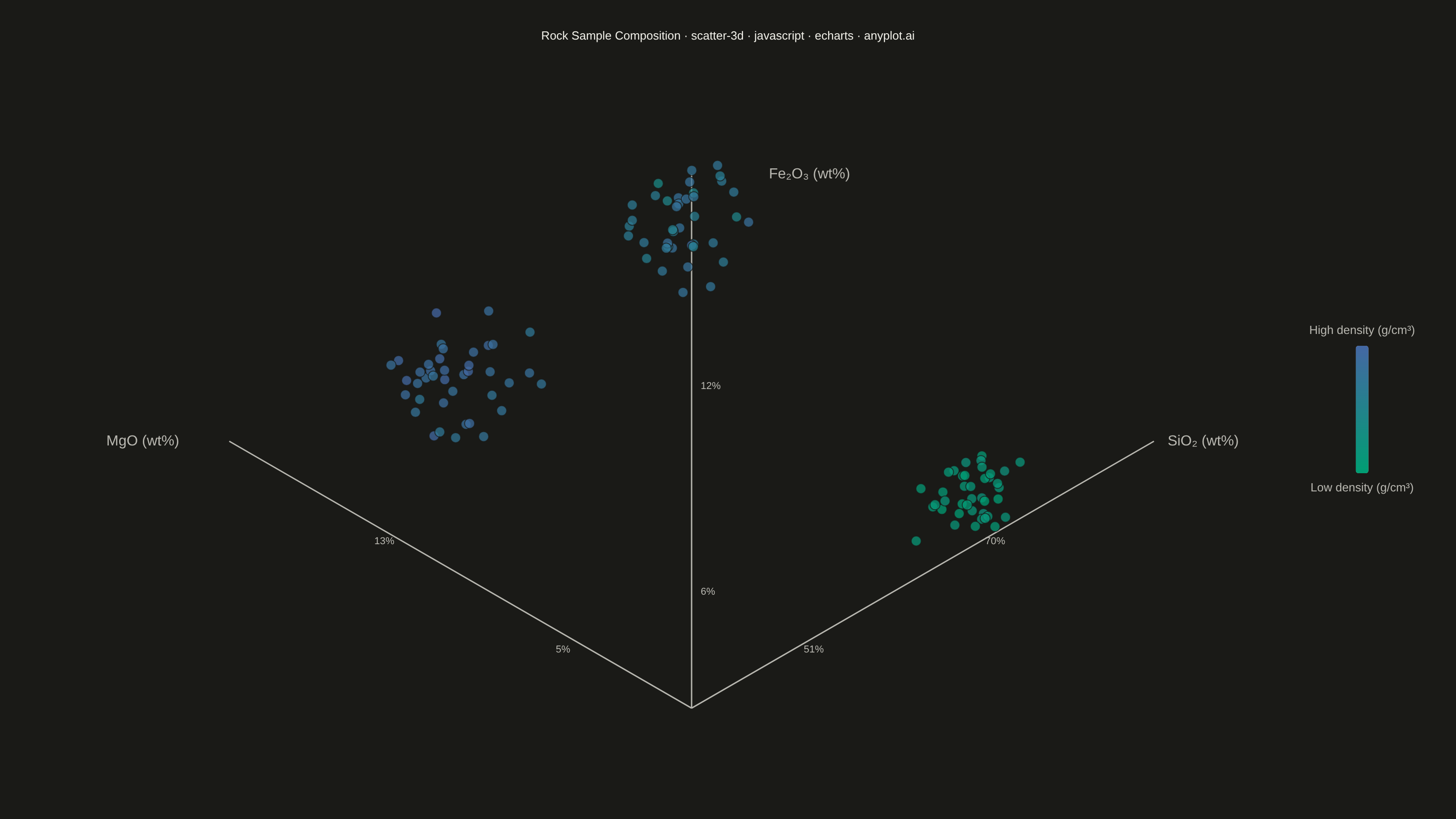
The same plot in 13 other libraries — JavaScript: Chart.js, D3.js, Highcharts, MUI X Charts; Python: Altair, Bokeh, lets-plot, Matplotlib, Plotly, Pygal, Seaborn; R: ggplot2; Julia: Makie.jl. Compare all 14 side by side: 3D Scatter Plot in Python, R, Julia and JavaScript.
A three-dimensional scatter plot that displays the relationship between three numeric variables by plotting points in 3D space. This visualization extends the classic 2D scatter plot to reveal patterns, clusters, and correlations across three dimensions simultaneously, making it invaluable for multivariate data exploration.
// anyplot.ai
// scatter-3d: 3D Scatter Plot
// Library: echarts 6.1.0 | JavaScript 22.23.2
// Quality: 85/100 | Created: 2026-09-10

//# anyplot-orientation: landscape
const t = window.ANYPLOT_TOKENS;
const size = window.ANYPLOT_SIZE;

// --- Deterministic PRNG (LCG + Box-Muller) -----------------------------------
let seed = 42;
function rand() {
  seed = (seed * 1664525 + 1013904223) % 4294967296;
  return seed / 4294967296;
}
function gaussian(mean, std) {
  const u1 = Math.max(rand(), 1e-9);
  const u2 = rand();
  return mean + std * Math.sqrt(-2 * Math.log(u1)) * Math.cos(2 * Math.PI * u2);
}

// --- Data: rock samples in 3D compositional space, density as 4th dimension -
// SiO2 / Fe2O3 / MgO (wt%) separate three igneous rock groups; density (g/cm3)
// is layered on top as a continuous color-encoded variable.
const clusters = [
  { n: 40, siO2: 50, fe2O3: 13, mgO: 5, density: 2.95, spread: [3, 0.9, 0.9, 0.05] },
  { n: 40, siO2: 72, fe2O3: 3, mgO: 1, density: 2.68, spread: [2.5, 0.6, 0.4, 0.03] },
  { n: 40, siO2: 46, fe2O3: 6, mgO: 13, density: 3.02, spread: [2.5, 0.8, 0.9, 0.04] },
];

const samples = [];
clusters.forEach((c) => {
  for (let i = 0; i < c.n; i++) {
    samples.push({
      siO2: gaussian(c.siO2, c.spread[0]),
      fe2O3: Math.max(0.2, gaussian(c.fe2O3, c.spread[1])),
      mgO: Math.max(0.1, gaussian(c.mgO, c.spread[2])),
      density: gaussian(c.density, c.spread[3]),
    });
  }
});

const siO2Range = [Math.min(...samples.map((s) => s.siO2)), Math.max(...samples.map((s) => s.siO2))];
const fe2O3Range = [Math.min(...samples.map((s) => s.fe2O3)), Math.max(...samples.map((s) => s.fe2O3))];
const mgORange = [Math.min(...samples.map((s) => s.mgO)), Math.max(...samples.map((s) => s.mgO))];
const densityRange = [Math.min(...samples.map((s) => s.density)), Math.max(...samples.map((s) => s.density))];

function norm(v, [lo, hi]) {
  return ((v - lo) / (hi - lo)) * 10;
}

// --- Isometric projection: (x, y, z) -> (screenX, screenY) ------------------
// Standard 30-degree axonometric projection: y is the vertical axis, x runs to
// the lower-right, z runs to the lower-left — the classic isometric layout.
const COS30 = Math.cos(Math.PI / 6);
const SIN30 = Math.sin(Math.PI / 6);
function project(nx, ny, nz) {
  return [(nx - nz) * COS30, (nx + nz) * SIN30 + ny];
}

const points = samples.map((s) => {
  const [px, py] = project(norm(s.siO2, siO2Range), norm(s.fe2O3, fe2O3Range), norm(s.mgO, mgORange));
  return [px, py, s.density, s.siO2, s.fe2O3, s.mgO];
});

// Axis guides run past the data extent (13 vs. the normalized max of 10) so
// the guide lines read as open-ended axes rather than a closed data-bound box.
const originP = project(0, 0, 0);
const xTip = project(13, 0, 0);
const yTip = project(0, 13, 0);
const zTip = project(0, 0, 13);

// --- Frame geometry: preserve the isometric angles by locking x/y to a
// single pixels-per-unit scale (echarts cartesian has no built-in aspect lock)
const allX = points.map((p) => p[0]).concat([originP[0], xTip[0], yTip[0], zTip[0]]);
const allY = points.map((p) => p[1]).concat([originP[1], xTip[1], yTip[1], zTip[1]]);
const padX = (Math.max(...allX) - Math.min(...allX)) * 0.12;
const padY = (Math.max(...allY) - Math.min(...allY)) * 0.08;
const xAxisMin = Math.min(...allX) - padX;
const xAxisMax = Math.max(...allX) + padX;
const yAxisMin = Math.min(...allY) - padY;
const yAxisMax = Math.max(...allY) + padY;

const marginTop = 110;
const marginBottom = 50;
const marginLeft = 130;
const marginRight = 210;
const availW = size.width - marginLeft - marginRight;
const availH = size.height - marginTop - marginBottom;
const dataW = xAxisMax - xAxisMin;
const dataH = yAxisMax - yAxisMin;
const gridScale = Math.min(availW / dataW, availH / dataH);
const gridWidth = dataW * gridScale;
const gridHeight = dataH * gridScale;
const gridLeft = marginLeft + (availW - gridWidth) / 2;
const gridTop = marginTop + (availH - gridHeight) / 2;

// --- Title (fontsize scaled to the 67-char baseline) -------------------------
const titleText = "Rock Sample Composition · scatter-3d · javascript · echarts · anyplot.ai";
const titleFontSize = Math.max(15, Math.round(22 * Math.min(1, 67 / titleText.length)));

// --- Init ---------------------------------------------------------------------
const chart = echarts.init(document.getElementById("container"));

// --- Option ---------------------------------------------------------------
const option = {
  animation: false,
  backgroundColor: "transparent",
  color: t.palette,
  title: {
    text: titleText,
    left: "center",
    top: 30,
    textStyle: { color: t.ink, fontSize: titleFontSize, fontWeight: "medium" },
  },
  tooltip: {
    trigger: "item",
    formatter: (params) => {
      if (!Array.isArray(params.data)) return "";
      const [, , density, siO2, fe2O3, mgO] = params.data;
      return (
        `SiO₂: ${siO2.toFixed(1)} wt%<br/>` +
        `Fe₂O₃: ${fe2O3.toFixed(1)} wt%<br/>` +
        `MgO: ${mgO.toFixed(1)} wt%<br/>` +
        `Density: ${density.toFixed(2)} g/cm³`
      );
    },
    backgroundColor: t.elevatedBg,
    borderColor: t.inkSoft,
    textStyle: { color: t.ink },
  },
  visualMap: {
    dimension: 2,
    min: densityRange[0],
    max: densityRange[1],
    inRange: { color: t.seq },
    orient: "vertical",
    right: 30,
    top: "middle",
    text: ["High density (g/cm³)", "Low density (g/cm³)"],
    textStyle: { color: t.inkSoft, fontSize: 13 },
    itemWidth: 14,
    itemHeight: 140,
  },
  grid: { left: gridLeft, top: gridTop, width: gridWidth, height: gridHeight },
  xAxis: {
    type: "value",
    min: xAxisMin,
    max: xAxisMax,
    show: false,
  },
  yAxis: {
    type: "value",
    min: yAxisMin,
    max: yAxisMax,
    show: false,
  },
  series: [
    {
      // Axis guides
      type: "line",
      data: [
        [originP[0], originP[1]],
        [xTip[0], xTip[1]],
      ],
      showSymbol: false,
      silent: true,
      lineStyle: { color: t.inkSoft, width: 1.5 },
      z: 1,
    },
    {
      type: "line",
      data: [
        [originP[0], originP[1]],
        [yTip[0], yTip[1]],
      ],
      showSymbol: false,
      silent: true,
      lineStyle: { color: t.inkSoft, width: 1.5 },
      z: 1,
    },
    {
      type: "line",
      data: [
        [originP[0], originP[1]],
        [zTip[0], zTip[1]],
      ],
      showSymbol: false,
      silent: true,
      lineStyle: { color: t.inkSoft, width: 1.5 },
      z: 1,
    },
    {
      // Rock samples, positioned by isometric projection, colored by density
      type: "scatter",
      data: points,
      symbolSize: 11,
      itemStyle: {
        opacity: 0.75,
        borderColor: t.pageBg,
        borderWidth: 1,
      },
      z: 2,
    },
  ],
};

chart.setOption(option);

// Axis labels, anchored to each guide's tip and nudged off the line itself —
// real data coordinates converted to pixels, not a decorative overlay.
const toPixel = (dataPoint) => chart.convertToPixel({ xAxisIndex: 0, yAxisIndex: 0 }, dataPoint);
const axisLabels = [
  { point: xTip, text: "SiO₂ (wt%)", dx: 15, dy: -8, font: "16px sans-serif" },
  { point: yTip, text: "Fe₂O₃ (wt%)", dx: 85, dy: -8, font: "16px sans-serif" },
  { point: zTip, text: "MgO (wt%)", dx: -135, dy: -8, font: "16px sans-serif" },
];

// Numeric tick labels partway along each guide (interpolated from that
// variable's real min/max) so the composition scale reads directly off the
// static PNG without needing the interactive tooltip.
function tickValue([lo, hi], frac) {
  return lo + (frac / 10) * (hi - lo);
}
const tickSpecs = [
  { axisVec: [1, 0, 0], range: siO2Range, ticks: [{ t: 3, dx: 6, dy: -2 }, { t: 8, dx: 10, dy: -8 }] },
  { axisVec: [0, 1, 0], range: fe2O3Range, ticks: [{ t: 3, dx: 10, dy: 2 }, { t: 8, dx: 10, dy: 2 }] },
  { axisVec: [0, 0, 1], range: mgORange, ticks: [{ t: 3, dx: -32, dy: -2 }, { t: 8, dx: -36, dy: -8 }] },
];
const tickLabels = tickSpecs.flatMap((spec) =>
  spec.ticks.map(({ t: frac, dx, dy }) => ({
    point: project(spec.axisVec[0] * frac, spec.axisVec[1] * frac, spec.axisVec[2] * frac),
    text: `${tickValue(spec.range, frac).toFixed(0)}%`,
    dx,
    dy,
    font: "11px sans-serif",
  }))
);

chart.setOption({
  graphic: [...axisLabels, ...tickLabels].map((a) => {
    const pixel = toPixel([a.point[0], a.point[1]]);
    return {
      type: "text",
      left: pixel[0] + a.dx,
      top: pixel[1] + a.dy,
      silent: true,
      style: { text: a.text, fill: t.inkSoft, font: a.font },
    };
  }),
});
Runnable source as JSON, for any HTTP client: https://api.anyplot.ai/specs/scatter-3d/echarts/code. Any spec id and library id listed in llms-full.txt fit the same URL shape; every URL below is complete and callable.
{
  "spec_id": "scatter-3d",
  "language": "javascript",
  "library": "echarts",
  "page": "https://anyplot.ai/scatter-3d/javascript/echarts",
  "hub": "https://anyplot.ai/scatter-3d",
  "code_json": "https://api.anyplot.ai/specs/scatter-3d/echarts/code",
  "spec_json": "https://api.anyplot.ai/specs/scatter-3d",
  "render_light_png": "https://storage.googleapis.com/anyplot-images/plots/scatter-3d/javascript/echarts/plot-light.png",
  "render_dark_png": "https://storage.googleapis.com/anyplot-images/plots/scatter-3d/javascript/echarts/plot-dark.png",
  "interactive_light_html": "https://storage.googleapis.com/anyplot-images/plots/scatter-3d/javascript/echarts/plot-light.html",
  "interactive_dark_html": "https://storage.googleapis.com/anyplot-images/plots/scatter-3d/javascript/echarts/plot-dark.html",
  "quality_score": 85.0,
  "license": "MIT",
  "guide": "https://anyplot.ai/llms.txt"
}
Part of 3D Scatter Plot on anyplot.ai.