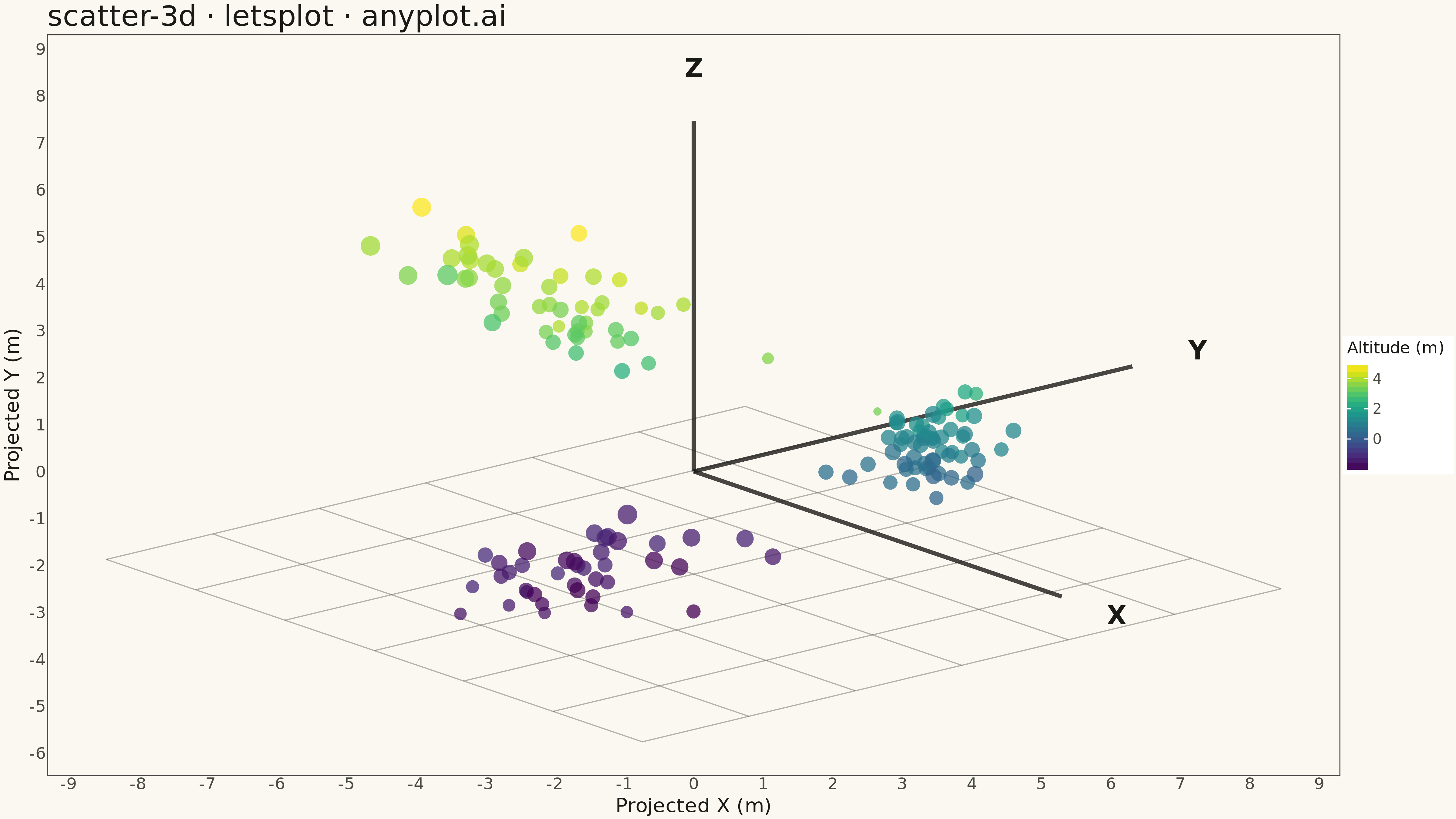
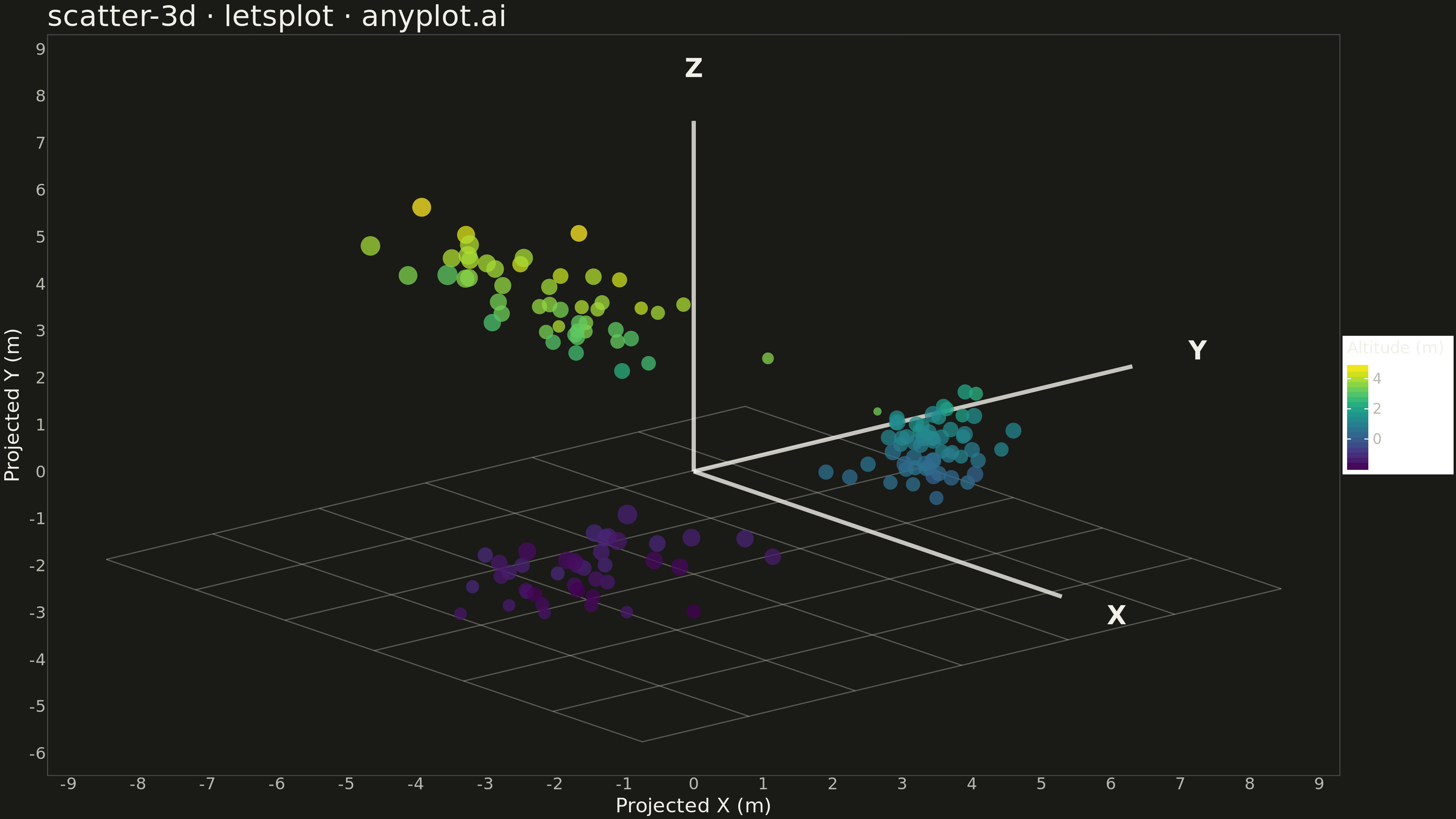
A three-dimensional scatter plot that displays the relationship between three numeric variables by plotting points in 3D space. This visualization extends the classic 2D scatter plot to reveal patterns, clusters, and correlations across three dimensions simultaneously, making it invaluable for multivariate data exploration.
""" anyplot.ai
scatter-3d: 3D Scatter Plot
Library: letsplot 4.9.0 | Python 3.13.13
Quality: 89/100 | Updated: 2026-05-08
"""

import numpy as np
import pandas as pd
from lets_plot import (
    LetsPlot,
    aes,
    element_blank,
    element_text,
    geom_point,
    geom_segment,
    geom_text,
    ggplot,
    ggsize,
    labs,
    layer_tooltips,
    scale_color_viridis,
    scale_size_identity,
    theme,
    theme_minimal,
)
from lets_plot.export import ggsave


LetsPlot.setup_html()

# Data - Simulated 3D spatial measurements (e.g., sensor readings in a volume)
np.random.seed(42)

# Create 3 distinct clusters with varied characteristics
n_points = 150

# Cluster 1: Dense spherical cluster (tight sensor group) - 60 points
n1 = 60
c1_x = np.random.randn(n1) * 0.5 + 3
c1_y = np.random.randn(n1) * 0.5 + 2
c1_z = np.random.randn(n1) * 0.5 + 1

# Cluster 2: Elongated ellipsoid (stretched along X) - 50 points
n2 = 50
c2_x = np.random.randn(n2) * 1.8 - 2
c2_y = np.random.randn(n2) * 0.4 - 1
c2_z = np.random.randn(n2) * 0.6 + 3.5

# Cluster 3: Flat disk (spread in X-Y plane, thin in Z) - 40 points
n3 = 40
c3_x = np.random.randn(n3) * 1.2 + 0.5
c3_y = np.random.randn(n3) * 1.2 - 2.5
c3_z = np.random.randn(n3) * 0.2 - 1.5

x = np.concatenate([c1_x, c2_x, c3_x])
y = np.concatenate([c1_y, c2_y, c3_y])
z = np.concatenate([c1_z, c2_z, c3_z])

# 3D to 2D isometric projection with rotation angles for good viewing
elev = np.radians(25)  # elevation angle
azim = np.radians(-50)  # azimuth angle

# Apply rotation: first around z-axis (azimuth), then x-axis (elevation)
cos_azim, sin_azim = np.cos(azim), np.sin(azim)
cos_elev, sin_elev = np.cos(elev), np.sin(elev)

x_rot = x * cos_azim - y * sin_azim
y_rot = x * sin_azim + y * cos_azim

# Project to 2D
x_proj = x_rot
y_proj = y_rot * sin_elev + z * cos_elev

# Depth for sorting (painter's algorithm - back to front)
depth = y_rot * cos_elev - z * sin_elev
depth_norm = (depth - depth.min()) / (depth.max() - depth.min())
point_sizes = 4 + depth_norm * 6  # perspective: closer points larger

# Create DataFrame and sort by depth
df = pd.DataFrame({"x_proj": x_proj, "y_proj": y_proj, "altitude": z, "depth": depth, "size": point_sizes})
df = df.sort_values("depth").reset_index(drop=True)

# Project axis lines from origin - extended to span full data range
# Calculate data bounds for axis sizing
data_range = max(x.max() - x.min(), y.max() - y.min(), z.max() - z.min())
axis_length = data_range * 0.8  # 80% of data range for visible axes

# Project origin to 2D
origin_x_rot = 0.0
origin_y_rot = 0.0
origin_x_proj = origin_x_rot
origin_y_proj = origin_y_rot * sin_elev + 0.0 * cos_elev

# Project axis endpoints (X, Y, Z directions from origin)
# X axis direction: (axis_length, 0, 0)
x_end_rot_x = axis_length * cos_azim
x_end_rot_y = axis_length * sin_azim
x_end_proj_x = x_end_rot_x
x_end_proj_y = x_end_rot_y * sin_elev

# Y axis direction: (0, axis_length, 0)
y_end_rot_x = -axis_length * sin_azim
y_end_rot_y = axis_length * cos_azim
y_end_proj_x = y_end_rot_x
y_end_proj_y = y_end_rot_y * sin_elev

# Z axis direction: (0, 0, axis_length)
z_end_proj_x = 0.0
z_end_proj_y = axis_length * cos_elev

axes_df = pd.DataFrame(
    {
        "x": [origin_x_proj, origin_x_proj, origin_x_proj],
        "y": [origin_y_proj, origin_y_proj, origin_y_proj],
        "xend": [x_end_proj_x, y_end_proj_x, z_end_proj_x],
        "yend": [x_end_proj_y, y_end_proj_y, z_end_proj_y],
        "axis": ["X", "Y", "Z"],
    }
)

# Axis label positions (slightly beyond axis endpoints)
label_offset = 1.15
axis_labels_df = pd.DataFrame(
    {
        "x": [x_end_proj_x * label_offset, y_end_proj_x * label_offset, z_end_proj_x],
        "y": [x_end_proj_y * label_offset, y_end_proj_y * label_offset, z_end_proj_y * label_offset],
        "label": ["X", "Y", "Z"],
    }
)

# Create floor grid (XY plane at z_min) for depth perception
z_floor = z.min() - 0.5
grid_size = 6
grid_step = 2.0
grid_lines = []
for i in range(-grid_size // 2, grid_size // 2 + 1):
    # Lines parallel to X axis
    start_x, start_y = i * grid_step, -grid_size // 2 * grid_step
    end_x, end_y = i * grid_step, grid_size // 2 * grid_step
    # Project start point
    sx_rot = start_x * cos_azim - start_y * sin_azim
    sy_rot = start_x * sin_azim + start_y * cos_azim
    sx_proj = sx_rot
    sy_proj = sy_rot * sin_elev + z_floor * cos_elev
    # Project end point
    ex_rot = end_x * cos_azim - end_y * sin_azim
    ey_rot = end_x * sin_azim + end_y * cos_azim
    ex_proj = ex_rot
    ey_proj = ey_rot * sin_elev + z_floor * cos_elev
    grid_lines.append({"x": sx_proj, "y": sy_proj, "xend": ex_proj, "yend": ey_proj})
    # Lines parallel to Y axis
    start_x, start_y = -grid_size // 2 * grid_step, i * grid_step
    end_x, end_y = grid_size // 2 * grid_step, i * grid_step
    sx_rot = start_x * cos_azim - start_y * sin_azim
    sy_rot = start_x * sin_azim + start_y * cos_azim
    sx_proj = sx_rot
    sy_proj = sy_rot * sin_elev + z_floor * cos_elev
    ex_rot = end_x * cos_azim - end_y * sin_azim
    ey_rot = end_x * sin_azim + end_y * cos_azim
    ex_proj = ex_rot
    ey_proj = ey_rot * sin_elev + z_floor * cos_elev
    grid_lines.append({"x": sx_proj, "y": sy_proj, "xend": ex_proj, "yend": ey_proj})

grid_df = pd.DataFrame(grid_lines)

# Create the plot
plot = (
    ggplot()
    # Floor grid first (behind everything)
    + geom_segment(
        data=grid_df, mapping=aes(x="x", y="y", xend="xend", yend="yend"), color="#CCCCCC", size=0.5, alpha=0.4
    )
    # Axis lines
    + geom_segment(
        data=axes_df, mapping=aes(x="x", y="y", xend="xend", yend="yend"), color="#555555", size=2.0, alpha=0.8
    )
    # Axis labels (X, Y, Z)
    + geom_text(
        data=axis_labels_df, mapping=aes(x="x", y="y", label="label"), color="#333333", size=14, fontface="bold"
    )
    # Data points
    + geom_point(
        data=df,
        mapping=aes(x="x_proj", y="y_proj", color="altitude", size="size"),
        alpha=0.75,
        tooltips=layer_tooltips().line("Altitude|@altitude").line("Depth|@depth"),
    )
    + scale_color_viridis(name="Altitude (m)", option="viridis")
    + scale_size_identity()
    + labs(x="Projected X (m)", y="Projected Y (m)", title="scatter-3d · letsplot · pyplots.ai")
    + theme_minimal()
    + theme(
        axis_title=element_text(size=22),
        axis_text=element_text(size=18),
        plot_title=element_text(size=32),  # Fixed: increased from 28 to 32 for optimal visibility
        legend_text=element_text(size=16),
        legend_title=element_text(size=18),
        panel_grid=element_blank(),
    )
    + ggsize(1600, 900)
)

# Save PNG (scale=3 gives 4800x2700)
ggsave(plot, "plot.png", path=".", scale=3)

# Save HTML for interactivity
ggsave(plot, "plot.html", path=".")
Runnable source as JSON, for any HTTP client: https://api.anyplot.ai/specs/scatter-3d/letsplot/code. Any spec id and library id listed in llms-full.txt fit the same URL shape; every URL below is complete and callable.
{
  "spec_id": "scatter-3d",
  "language": "python",
  "library": "letsplot",
  "page": "https://anyplot.ai/scatter-3d/python/letsplot",
  "hub": "https://anyplot.ai/scatter-3d",
  "code_json": "https://api.anyplot.ai/specs/scatter-3d/letsplot/code",
  "spec_json": "https://api.anyplot.ai/specs/scatter-3d",
  "render_light_png": "https://storage.googleapis.com/anyplot-images/plots/scatter-3d/python/letsplot/plot-light.png",
  "render_dark_png": "https://storage.googleapis.com/anyplot-images/plots/scatter-3d/python/letsplot/plot-dark.png",
  "interactive_light_html": "https://storage.googleapis.com/anyplot-images/plots/scatter-3d/python/letsplot/plot-light.html",
  "interactive_dark_html": "https://storage.googleapis.com/anyplot-images/plots/scatter-3d/python/letsplot/plot-dark.html",
  "quality_score": 89.0,
  "license": "MIT",
  "guide": "https://anyplot.ai/llms.txt"
}
Part of 3D Scatter Plot on anyplot.ai.