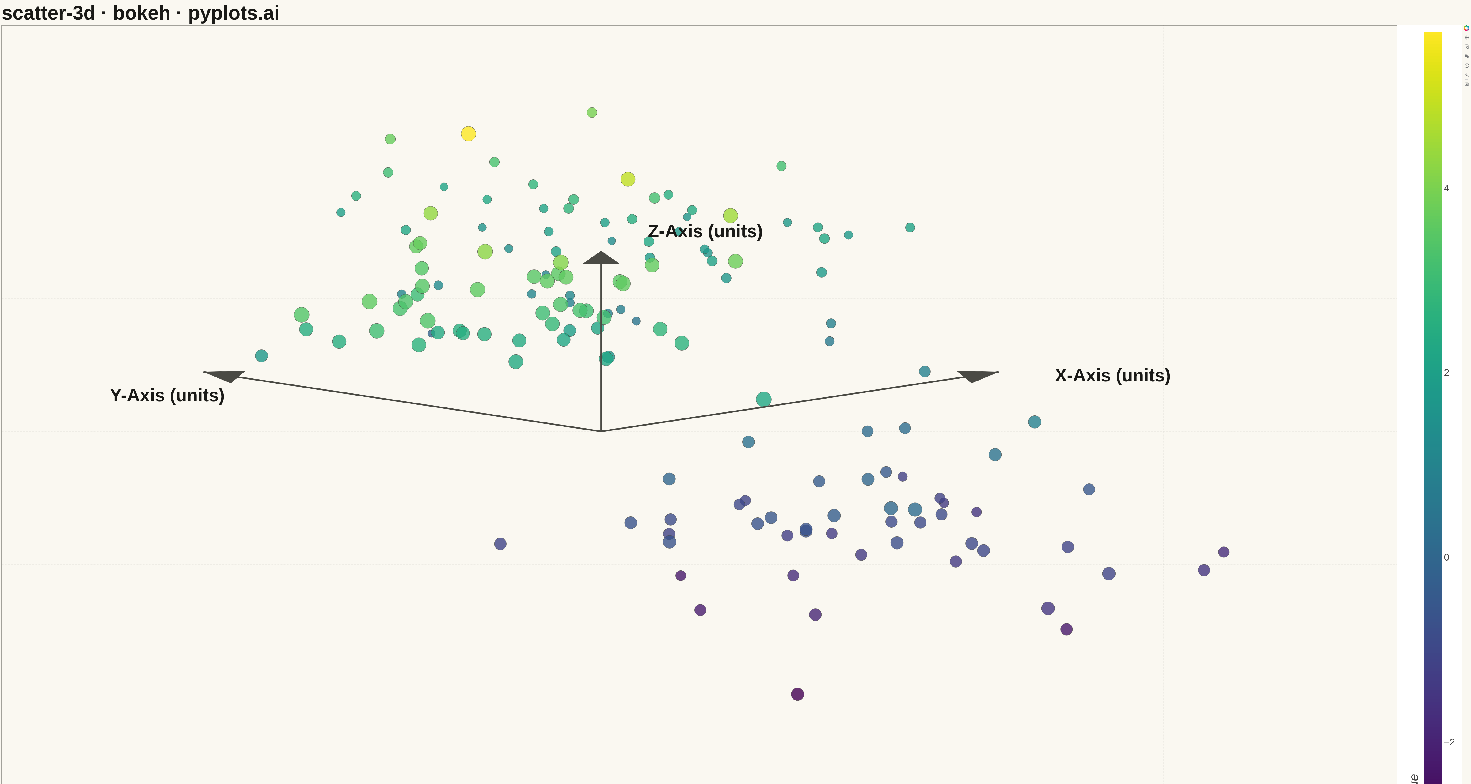
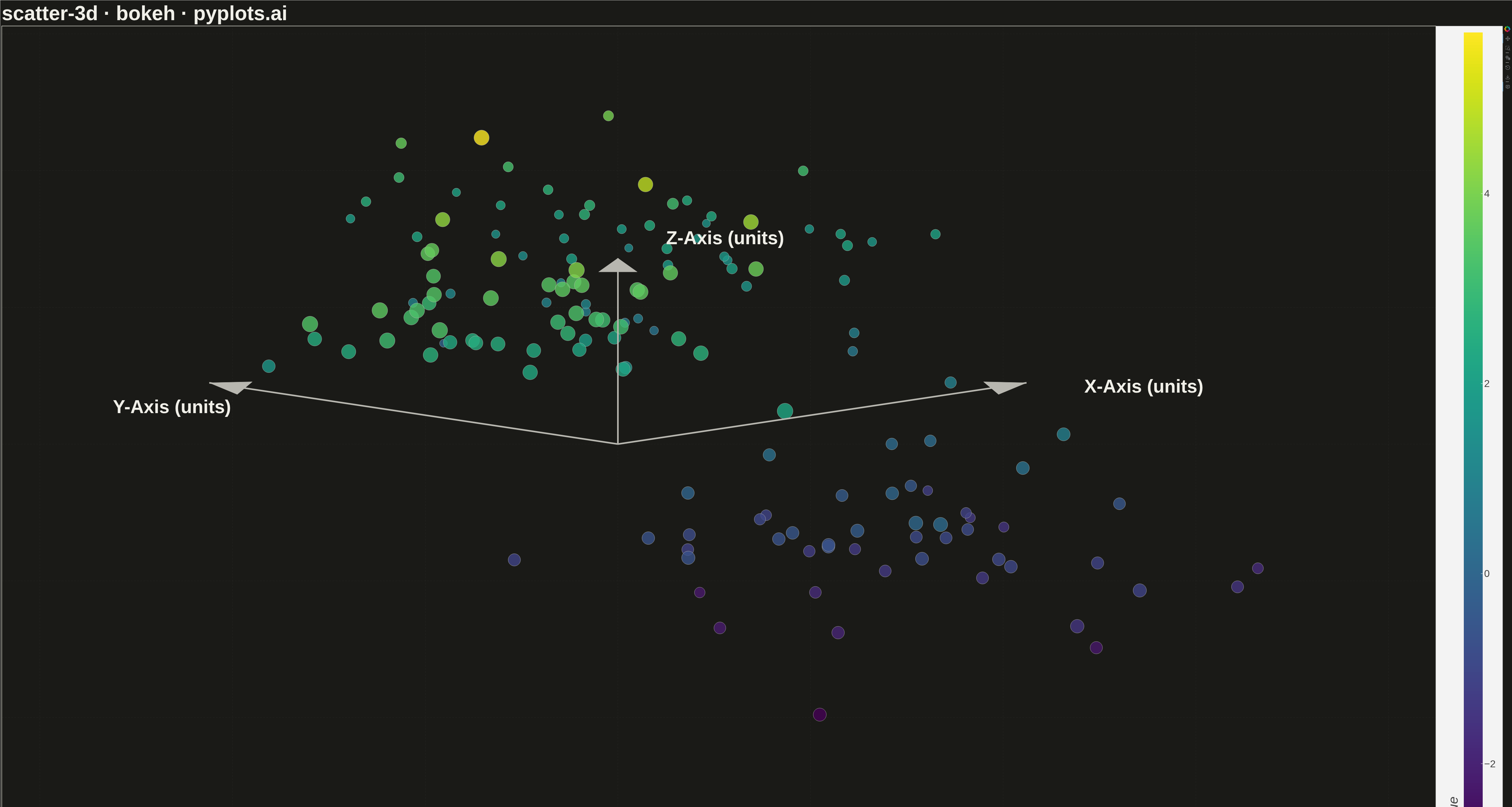
A three-dimensional scatter plot that displays the relationship between three numeric variables by plotting points in 3D space. This visualization extends the classic 2D scatter plot to reveal patterns, clusters, and correlations across three dimensions simultaneously, making it invaluable for multivariate data exploration.
""" anyplot.ai
scatter-3d: 3D Scatter Plot
Library: bokeh 3.9.0 | Python 3.13.13
Quality: 87/100 | Updated: 2026-05-08
"""

import os
import time
from pathlib import Path

import numpy as np
from bokeh.io import output_file, save
from bokeh.models import ColorBar, ColumnDataSource, Label, LinearColorMapper, Range1d
from bokeh.palettes import Viridis256
from bokeh.plotting import figure
from bokeh.resources import CDN
from selenium import webdriver
from selenium.webdriver.chrome.options import Options


# Theme tokens (read from environment, default light)
THEME = os.getenv("ANYPLOT_THEME", "light")
PAGE_BG = "#FAF8F1" if THEME == "light" else "#1A1A17"
ELEVATED_BG = "#FFFDF6" if THEME == "light" else "#242420"
INK = "#1A1A17" if THEME == "light" else "#F0EFE8"
INK_SOFT = "#4A4A44" if THEME == "light" else "#B8B7B0"

# Data - create 3D clustered data demonstrating spatial relationships
np.random.seed(42)

# Generate 3 clusters in 3D space (150 points total)
n_per_cluster = 50

# Cluster 1: centered at (2, 2, 2)
x1 = np.random.randn(n_per_cluster) * 0.8 + 2
y1 = np.random.randn(n_per_cluster) * 0.8 + 2
z1 = np.random.randn(n_per_cluster) * 0.8 + 2

# Cluster 2: centered at (-2, -1, 3)
x2 = np.random.randn(n_per_cluster) * 0.7 - 2
y2 = np.random.randn(n_per_cluster) * 0.7 - 1
z2 = np.random.randn(n_per_cluster) * 0.7 + 3

# Cluster 3: centered at (0, -2, -1)
x3 = np.random.randn(n_per_cluster) * 0.9
y3 = np.random.randn(n_per_cluster) * 0.9 - 2
z3 = np.random.randn(n_per_cluster) * 0.9 - 1

# Combine all clusters
x = np.concatenate([x1, x2, x3])
y = np.concatenate([y1, y2, y3])
z = np.concatenate([z1, z2, z3])

# 3D to 2D isometric projection (elevation=25°, azimuth=45°)
elev_rad = np.radians(25)
azim_rad = np.radians(45)

# Rotation around z-axis (azimuth)
x_rot = x * np.cos(azim_rad) - y * np.sin(azim_rad)
y_rot = x * np.sin(azim_rad) + y * np.cos(azim_rad)

# Rotation around x-axis (elevation) and project to 2D
x_proj = x_rot
z_proj = y_rot * np.sin(elev_rad) + z * np.cos(elev_rad)

# Calculate depth for size scaling and sorting (points further away are smaller)
depth = y_rot * np.cos(elev_rad) - z * np.sin(elev_rad)
depth_normalized = (depth - depth.min()) / (depth.max() - depth.min())

# Sort by depth (back to front) so front points render on top
sort_idx = np.argsort(-depth)  # Sort descending (back first)
x_proj_sorted = x_proj[sort_idx]
z_proj_sorted = z_proj[sort_idx]
z_sorted = z[sort_idx]
depth_sorted = depth_normalized[sort_idx]

# Scale marker size based on depth (25-50 for improved visibility at 4800x2700)
sizes = 25 + (1 - depth_sorted) * 25

# Color mapping using Z value (fourth dimension via color)
z_min, z_max = z.min(), z.max()
color_mapper = LinearColorMapper(palette=Viridis256, low=z_min, high=z_max)

# Map z values to colors
colors = []
for z_val in z_sorted:
    idx = int((z_val - z_min) / (z_max - z_min) * 255)
    idx = max(0, min(255, idx))
    colors.append(Viridis256[idx])

# Create ColumnDataSource
source = ColumnDataSource(
    data={"x": x_proj_sorted, "y": z_proj_sorted, "size": sizes, "color": colors, "z_value": z_sorted}
)

# Create Bokeh figure with interactive tools
p = figure(
    width=4800,
    height=2700,
    title="scatter-3d · bokeh · pyplots.ai",
    toolbar_location="right",
    tools="pan,wheel_zoom,box_zoom,reset,save",
)

# Draw scatter points with improved size for depth perception
p.scatter(x="x", y="y", size="size", color="color", alpha=0.8, line_color=INK_SOFT, line_width=1, source=source)

# Set appropriate ranges with padding - balanced layout
x_min, x_max = x_proj.min(), x_proj.max()
y_min, y_max = z_proj.min(), z_proj.max()
x_pad = (x_max - x_min) * 0.15
y_pad = (y_max - y_min) * 0.15

# Center the data in the plot area with balanced padding
p.x_range = Range1d(x_min - x_pad * 1.8, x_max + x_pad * 1.2)
p.y_range = Range1d(y_min - y_pad * 1.5, y_max + y_pad)

# Hide default axes for cleaner 3D projection look
p.xaxis.visible = False
p.yaxis.visible = False

# Custom 3D axis lines positioned at the projected origin
origin_3d_x, origin_3d_y, origin_3d_z = 0, 0, 0
origin_x_rot = origin_3d_x * np.cos(azim_rad) - origin_3d_y * np.sin(azim_rad)
origin_y_rot = origin_3d_x * np.sin(azim_rad) + origin_3d_y * np.cos(azim_rad)
origin_x = origin_x_rot
origin_y = origin_y_rot * np.sin(elev_rad) + origin_3d_z * np.cos(elev_rad)

# Axis styling - theme-adaptive
axis_color = INK_SOFT
axis_width = 5
axis_length = 3.0

# Project 3D axis endpoints to 2D
# X-axis: point (axis_length, 0, 0)
x_end_x_rot = axis_length * np.cos(azim_rad)
x_end_y_rot = axis_length * np.sin(azim_rad)
x_axis_end_x = x_end_x_rot
x_axis_end_y = x_end_y_rot * np.sin(elev_rad)

# Y-axis: point (0, axis_length, 0)
y_end_x_rot = -axis_length * np.sin(azim_rad)
y_end_y_rot = axis_length * np.cos(azim_rad)
y_axis_end_x = y_end_x_rot
y_axis_end_y = y_end_y_rot * np.sin(elev_rad)

# Z-axis: point (0, 0, axis_length)
z_axis_end_x = origin_x
z_axis_end_y = origin_y + axis_length * np.cos(elev_rad)

# Draw axis lines from projected origin
p.line(x=[origin_x, x_axis_end_x], y=[origin_y, x_axis_end_y], line_color=axis_color, line_width=axis_width)
p.line(x=[origin_x, y_axis_end_x], y=[origin_y, y_axis_end_y], line_color=axis_color, line_width=axis_width)
p.line(x=[origin_x, z_axis_end_x], y=[origin_y, z_axis_end_y], line_color=axis_color, line_width=axis_width)

# Add axis arrows (small triangles at the end of each axis)
arrow_size = 0.2

# X-axis arrow
x_dir = np.array([x_axis_end_x - origin_x, x_axis_end_y - origin_y])
x_dir = x_dir / np.linalg.norm(x_dir)
x_perp = np.array([-x_dir[1], x_dir[0]])
p.patch(
    x=[
        x_axis_end_x,
        x_axis_end_x - arrow_size * x_dir[0] + arrow_size * 0.5 * x_perp[0],
        x_axis_end_x - arrow_size * x_dir[0] - arrow_size * 0.5 * x_perp[0],
    ],
    y=[
        x_axis_end_y,
        x_axis_end_y - arrow_size * x_dir[1] + arrow_size * 0.5 * x_perp[1],
        x_axis_end_y - arrow_size * x_dir[1] - arrow_size * 0.5 * x_perp[1],
    ],
    fill_color=axis_color,
    line_color=axis_color,
)

# Y-axis arrow
y_dir = np.array([y_axis_end_x - origin_x, y_axis_end_y - origin_y])
y_dir = y_dir / np.linalg.norm(y_dir)
y_perp = np.array([-y_dir[1], y_dir[0]])
p.patch(
    x=[
        y_axis_end_x,
        y_axis_end_x - arrow_size * y_dir[0] + arrow_size * 0.5 * y_perp[0],
        y_axis_end_x - arrow_size * y_dir[0] - arrow_size * 0.5 * y_perp[0],
    ],
    y=[
        y_axis_end_y,
        y_axis_end_y - arrow_size * y_dir[1] + arrow_size * 0.5 * y_perp[1],
        y_axis_end_y - arrow_size * y_dir[1] - arrow_size * 0.5 * y_perp[1],
    ],
    fill_color=axis_color,
    line_color=axis_color,
)

# Z-axis arrow
z_dir = np.array([z_axis_end_x - origin_x, z_axis_end_y - origin_y])
z_dir = z_dir / np.linalg.norm(z_dir)
z_perp = np.array([-z_dir[1], z_dir[0]])
p.patch(
    x=[
        z_axis_end_x,
        z_axis_end_x - arrow_size * z_dir[0] + arrow_size * 0.5 * z_perp[0],
        z_axis_end_x - arrow_size * z_dir[0] - arrow_size * 0.5 * z_perp[0],
    ],
    y=[
        z_axis_end_y,
        z_axis_end_y - arrow_size * z_dir[1] + arrow_size * 0.5 * z_perp[1],
        z_axis_end_y - arrow_size * z_dir[1] - arrow_size * 0.5 * z_perp[1],
    ],
    fill_color=axis_color,
    line_color=axis_color,
)

# Add descriptive axis labels with units - theme-adaptive text
x_label = Label(
    x=x_axis_end_x + 0.3,
    y=x_axis_end_y - 0.2,
    text="X-Axis (units)",
    text_font_size="44pt",
    text_color=INK,
    text_font_style="bold",
)
p.add_layout(x_label)

y_label = Label(
    x=y_axis_end_x - 0.5,
    y=y_axis_end_y - 0.5,
    text="Y-Axis (units)",
    text_font_size="44pt",
    text_color=INK,
    text_font_style="bold",
)
p.add_layout(y_label)

z_label = Label(
    x=z_axis_end_x + 0.25,
    y=z_axis_end_y + 0.15,
    text="Z-Axis (units)",
    text_font_size="44pt",
    text_color=INK,
    text_font_style="bold",
)
p.add_layout(z_label)

# Add color bar for Z-value scale (clarified title)
color_bar = ColorBar(
    color_mapper=color_mapper,
    width=60,
    location=(0, 0),
    title="Z-Value",
    title_text_font_size="32pt",
    major_label_text_font_size="24pt",
    title_standoff=20,
    margin=40,
    padding=20,
)
p.add_layout(color_bar, "right")

# Title styling for large canvas - theme-adaptive
p.title.text_font_size = "48pt"
p.title.text_font_style = "bold"
p.title.text_color = INK

# Grid styling - much more subtle to not conflict with 3D axes
p.xgrid.grid_line_color = INK
p.ygrid.grid_line_color = INK
p.xgrid.grid_line_alpha = 0.05
p.ygrid.grid_line_alpha = 0.05
p.xgrid.grid_line_dash = [6, 4]
p.ygrid.grid_line_dash = [6, 4]

# Background and border styling - theme-adaptive
p.background_fill_color = PAGE_BG
p.border_fill_color = PAGE_BG
p.outline_line_color = INK_SOFT
p.min_border_right = 220

# Save HTML output
output_file(f"plot-{THEME}.html")
save(p, resources=CDN, title="scatter-3d · bokeh · pyplots.ai")

# Screenshot with Selenium/Chrome for PNG export
W, H = 4800, 2700
opts = Options()
for arg in (
    "--headless=new",
    "--no-sandbox",
    "--disable-dev-shm-usage",
    "--disable-gpu",
    f"--window-size={W},{H}",
    "--hide-scrollbars",
):
    opts.add_argument(arg)

driver = webdriver.Chrome(options=opts)
driver.set_window_size(W, H)
driver.get(f"file://{Path(f'plot-{THEME}.html').resolve()}")
time.sleep(3)  # Let Bokeh's JS render the canvas
driver.save_screenshot(f"plot-{THEME}.png")
driver.quit()
Runnable source as JSON, for any HTTP client: https://api.anyplot.ai/specs/scatter-3d/bokeh/code. Any spec id and library id listed in llms-full.txt fit the same URL shape; every URL below is complete and callable.
{
  "spec_id": "scatter-3d",
  "language": "python",
  "library": "bokeh",
  "page": "https://anyplot.ai/scatter-3d/python/bokeh",
  "hub": "https://anyplot.ai/scatter-3d",
  "code_json": "https://api.anyplot.ai/specs/scatter-3d/bokeh/code",
  "spec_json": "https://api.anyplot.ai/specs/scatter-3d",
  "render_light_png": "https://storage.googleapis.com/anyplot-images/plots/scatter-3d/python/bokeh/plot-light.png",
  "render_dark_png": "https://storage.googleapis.com/anyplot-images/plots/scatter-3d/python/bokeh/plot-dark.png",
  "interactive_light_html": "https://storage.googleapis.com/anyplot-images/plots/scatter-3d/python/bokeh/plot-light.html",
  "interactive_dark_html": "https://storage.googleapis.com/anyplot-images/plots/scatter-3d/python/bokeh/plot-dark.html",
  "quality_score": 87.0,
  "license": "MIT",
  "guide": "https://anyplot.ai/llms.txt"
}
Part of 3D Scatter Plot on anyplot.ai.