The same plot in 13 other libraries — Python: Altair, Bokeh, lets-plot, Matplotlib, Plotly, Pygal, Seaborn; Julia: Makie.jl; JavaScript: Chart.js, D3.js, Apache ECharts, Highcharts, MUI X Charts. Compare all 14 side by side: 3D Scatter Plot in Python, R, Julia and JavaScript.
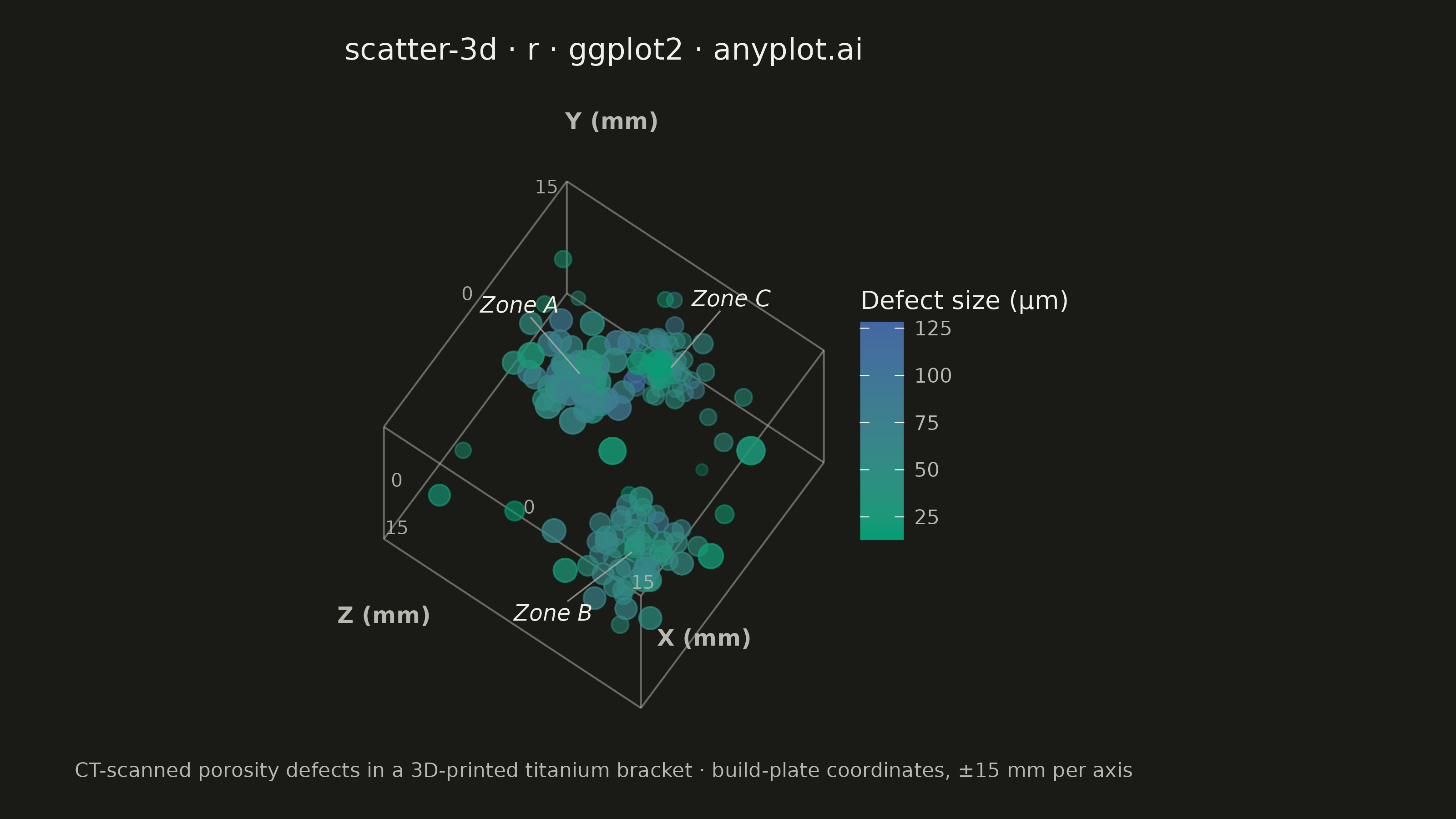
A three-dimensional scatter plot that displays the relationship between three numeric variables by plotting points in 3D space. This visualization extends the classic 2D scatter plot to reveal patterns, clusters, and correlations across three dimensions simultaneously, making it invaluable for multivariate data exploration.
#' anyplot.ai
#' scatter-3d: 3D Scatter Plot
#' Library: ggplot2 3.5.1 | R 4.4.1
#' Quality: 91/100 | Created: 2026-09-10

library(ggplot2)
library(dplyr)
library(tibble)
library(scales)
library(ragg)

set.seed(42)

# --- Theme tokens ------------------------------------------------------------
THEME            <- Sys.getenv("ANYPLOT_THEME", "light")
PAGE_BG          <- if (THEME == "light") "#FAF8F1" else "#1A1A17"
INK              <- if (THEME == "light") "#1A1A17" else "#F0EFE8"
INK_SOFT         <- if (THEME == "light") "#4A4A44" else "#B8B7B0"
IMPRINT_SEQ_LOW  <- "#009E73"
IMPRINT_SEQ_HIGH <- "#4467A3"

# --- Data: CT-scanned porosity defects inside a 3D-printed titanium bracket -
# Three weak layer-adhesion zones plus scattered background porosity, in
# build-plate coordinates (mm). Defect size (micrometers) is the 4th variable.
n_zone      <- 55
zone_x      <- c(-9, 7, 1)
zone_y      <- c(6, -7, 9)
zone_z      <- c(5, 7, -6)
zone_spread <- c(2.6, 3.1, 2.3)

x <- c(
  rnorm(n_zone, zone_x[1], zone_spread[1]),
  rnorm(n_zone, zone_x[2], zone_spread[2]),
  rnorm(n_zone, zone_x[3], zone_spread[3]),
  runif(20, -15, 15)
)
y <- c(
  rnorm(n_zone, zone_y[1], zone_spread[1]),
  rnorm(n_zone, zone_y[2], zone_spread[2]),
  rnorm(n_zone, zone_y[3], zone_spread[3]),
  runif(20, -15, 15)
)
z <- c(
  rnorm(n_zone, zone_z[1], zone_spread[1]),
  rnorm(n_zone, zone_z[2], zone_spread[2]),
  rnorm(n_zone, zone_z[3], zone_spread[3]),
  runif(20, -15, 15)
)
defect_size_um <- c(
  rgamma(n_zone, shape = 6, scale = 8) + 15,
  rgamma(n_zone, shape = 5, scale = 7) + 15,
  rgamma(n_zone, shape = 7, scale = 6) + 15,
  rgamma(20, shape = 2, scale = 6) + 10
)

# --- Orthographic projection (azimuth 35°, elevation 20°) --------------------
# ggplot2 has no native 3D geom, so the third axis is folded into 2D screen
# space via a standard rotate-then-project transform (the same math a 3D
# chart library applies internally), rendered with geom_point/geom_segment.
az <- 35 * pi / 180
el <- 20 * pi / 180

project <- function(px, py, pz) {
  x_rot <- px * cos(az) + py * sin(az)
  y_rot <- -px * sin(az) + py * cos(az)
  list(proj_x = x_rot, proj_y = y_rot * cos(el) - pz * sin(el))
}

proj  <- project(x, y, z)
depth <- (-x * sin(az) + y * cos(az)) * sin(el) + z * cos(el) # larger = closer

points_df <- tibble(
  proj_x         = proj$proj_x,
  proj_y         = proj$proj_y,
  depth          = depth,
  defect_size_um = defect_size_um
) %>%
  mutate(
    depth_norm  = rescale(depth, to = c(0, 1)),
    # Power curve (not linear) spreads size/alpha further apart across depth,
    # so overlapping points in the densest cluster cores separate more clearly.
    point_size  = 1.8 + depth_norm^1.3 * 3.0,
    point_alpha = 0.32 + depth_norm^1.3 * 0.55
  ) %>%
  arrange(depth)

# --- Bounding-box wireframe (static 3D reference frame) ----------------------
pad <- 1.15
xr  <- range(x) * pad
yr  <- range(y) * pad
zr  <- range(z) * pad

corners       <- expand.grid(cx = xr, cy = yr, cz = zr)
corner_proj   <- project(corners$cx, corners$cy, corners$cz)
corners$proj_x <- corner_proj$proj_x
corners$proj_y <- corner_proj$proj_y

edge_from <- c(1, 3, 5, 7, 1, 2, 5, 6, 1, 2, 3, 4)
edge_to   <- c(2, 4, 6, 8, 3, 4, 7, 8, 5, 6, 7, 8)
edges_df <- tibble(
  x    = corners$proj_x[edge_from],
  y    = corners$proj_y[edge_from],
  xend = corners$proj_x[edge_to],
  yend = corners$proj_y[edge_to]
)

# --- Axis labels, extended past the box tips along their own direction -------
tip_idx  <- c(2, 3, 5) # X, Y, Z edges all start at corner 1
dir_x    <- corners$proj_x[tip_idx] - corners$proj_x[1]
dir_y    <- corners$proj_y[tip_idx] - corners$proj_y[1]
dir_len  <- sqrt(dir_x^2 + dir_y^2)
unit_x   <- dir_x / dir_len
unit_y   <- dir_y / dir_len
label_gap <- 8.2 # generous clearance so axis titles clear nearby data points

axis_labels <- tibble(
  label = c("X (mm)", "Y (mm)", "Z (mm)"),
  x     = corners$proj_x[tip_idx] + unit_x * label_gap,
  y     = corners$proj_y[tip_idx] + unit_y * label_gap
)

# --- Numeric tick references along each axis edge (mid/high mm values) -------
# Reviewers noted the box had no coordinate scale; nudge each tick label
# perpendicular to its edge so it reads as a ruler mark, not edge clutter.
# The low end (-15) sits at the shared tri-axis corner for all three axes, so
# it is skipped here — labeling it three times over would just overlap.
tick_vals   <- c(0, 15)
tick_nudge  <- 1.4
tick_x_proj <- project(tick_vals, rep(yr[1], 2), rep(zr[1], 2))
tick_y_proj <- project(rep(xr[1], 2), tick_vals, rep(zr[1], 2))
tick_z_proj <- project(rep(xr[1], 2), rep(yr[1], 2), tick_vals)

tick_labels <- tibble(
  label = as.character(rep(tick_vals, 3)),
  x = c(tick_x_proj$proj_x, tick_y_proj$proj_x, tick_z_proj$proj_x) -
    rep(unit_y, each = 2) * tick_nudge,
  y = c(tick_x_proj$proj_y, tick_y_proj$proj_y, tick_z_proj$proj_y) +
    rep(unit_x, each = 2) * tick_nudge
)

# --- Zone callouts, linking the projected scatter back to the CT-scan narrative
# Each callout sits well outside its dense point cluster, with a thin leader
# segment back to the cluster centroid, so the label never lands on top of
# 55+ overlapping alpha-blended points. Offsets are hand-tuned per zone (not
# a single radial push-out) because Zone B's cluster sits almost exactly
# along the same sightline as the X-axis tip/title, so pushing it further
# out along that line would just collide with "X (mm)" instead.
zone_proj    <- project(zone_x, zone_y, zone_z)
zone_off_x   <- c(-6.5, -8.5, 6.5)
zone_off_y   <- c(7.5, -6.5, 7.5)

zone_labels <- tibble(
  label = c("Zone A", "Zone B", "Zone C"),
  x     = zone_proj$proj_x + zone_off_x,
  y     = zone_proj$proj_y + zone_off_y
)

zone_leaders <- tibble(
  x    = zone_proj$proj_x,
  y    = zone_proj$proj_y,
  xend = zone_proj$proj_x + zone_off_x * 0.82,
  yend = zone_proj$proj_y + zone_off_y * 0.82
)

# --- Plot ---------------------------------------------------------------------
p <- ggplot() +
  geom_segment(
    data = edges_df,
    aes(x = x, y = y, xend = xend, yend = yend),
    color = INK_SOFT, linewidth = 0.35, alpha = 0.5
  ) +
  geom_point(
    data = points_df,
    aes(x = proj_x, y = proj_y, color = defect_size_um,
        size = point_size, alpha = point_alpha)
  ) +
  geom_text(
    data = tick_labels,
    aes(x = x, y = y, label = label),
    color = INK_SOFT, size = 2.6, alpha = 0.9
  ) +
  geom_text(
    data = axis_labels,
    aes(x = x, y = y, label = label),
    color = INK_SOFT, size = 3.2, fontface = "bold"
  ) +
  geom_segment(
    data = zone_leaders,
    aes(x = x, y = y, xend = xend, yend = yend),
    color = INK_SOFT, linewidth = 0.3, alpha = 0.7
  ) +
  geom_text(
    data = zone_labels,
    aes(x = x, y = y, label = label),
    color = INK, size = 3.1, fontface = "italic"
  ) +
  scale_color_gradient(low = IMPRINT_SEQ_LOW, high = IMPRINT_SEQ_HIGH,
                        name = "Defect size (µm)") +
  scale_size_identity() +
  scale_alpha_identity() +
  coord_fixed(ratio = 1, clip = "off") +
  labs(
    title   = "scatter-3d · r · ggplot2 · anyplot.ai",
    caption = "CT-scanned porosity defects in a 3D-printed titanium bracket · build-plate coordinates, ±15 mm per axis"
  ) +
  theme_void(base_size = 8) +
  theme(
    plot.background   = element_rect(fill = PAGE_BG, color = PAGE_BG),
    panel.background  = element_rect(fill = PAGE_BG, color = NA),
    plot.title        = element_text(color = INK, size = 12, hjust = 0.5,
                                      margin = margin(b = 10)),
    plot.caption      = element_text(color = INK_SOFT, size = 8, hjust = 0.5,
                                      margin = margin(t = 10)),
    legend.title      = element_text(color = INK, size = 10),
    legend.text       = element_text(color = INK_SOFT, size = 8),
    legend.position   = "right",
    plot.margin       = margin(15, 25, 15, 15)
  )

# --- Save (PNG, both themes) ---------------------------------------------------
ggsave(
  filename = sprintf("plot-%s.png", THEME),
  plot     = p,
  device   = ragg::agg_png,
  width    = 8,
  height   = 4.5,
  units    = "in",
  dpi      = 400
)
Runnable source as JSON, for any HTTP client: https://api.anyplot.ai/specs/scatter-3d/ggplot2/code. Any spec id and library id listed in llms-full.txt fit the same URL shape; every URL below is complete and callable.
{
  "spec_id": "scatter-3d",
  "language": "r",
  "library": "ggplot2",
  "page": "https://anyplot.ai/scatter-3d/r/ggplot2",
  "hub": "https://anyplot.ai/scatter-3d",
  "code_json": "https://api.anyplot.ai/specs/scatter-3d/ggplot2/code",
  "spec_json": "https://api.anyplot.ai/specs/scatter-3d",
  "render_light_png": "https://storage.googleapis.com/anyplot-images/plots/scatter-3d/r/ggplot2/plot-light.png",
  "render_dark_png": "https://storage.googleapis.com/anyplot-images/plots/scatter-3d/r/ggplot2/plot-dark.png",
  "quality_score": 91.0,
  "license": "MIT",
  "guide": "https://anyplot.ai/llms.txt"
}
Part of 3D Scatter Plot on anyplot.ai.