The same plot in 14 other libraries — JavaScript: Chart.js, D3.js, Highcharts, MUI X Charts; Python: Altair, Bokeh, lets-plot, Matplotlib, Plotly, plotnine, Pygal, Seaborn; R: ggplot2; Julia: Makie.jl. Compare all 15 side by side: Annotated Scatter Plot with Text Labels in Python, R, Julia and JavaScript.
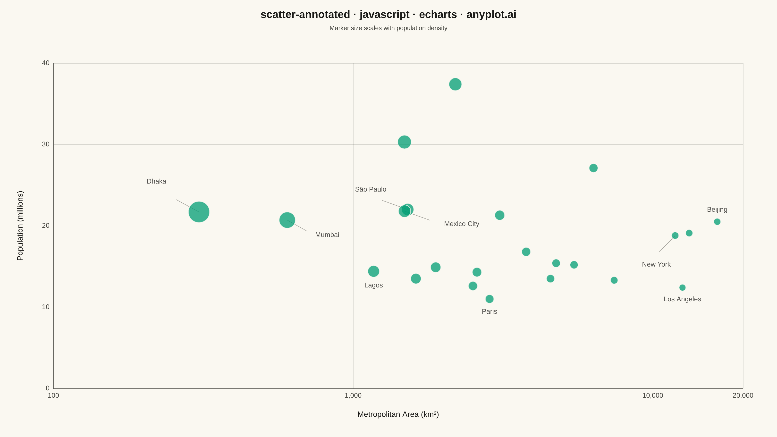
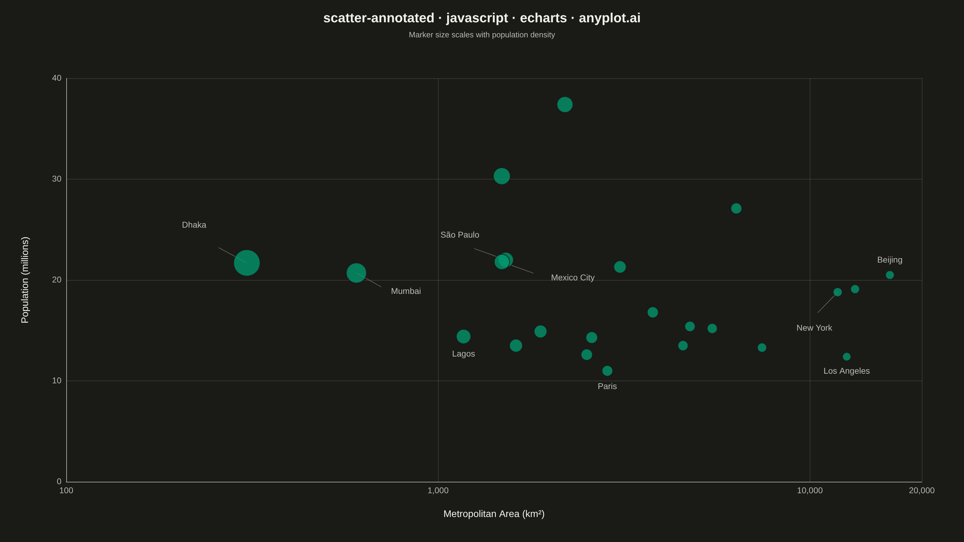
A scatter plot where each data point can have a text label annotation, useful for identifying specific points of interest. This visualization enhances basic scatter plots by adding contextual information directly on the chart, making it easy to highlight outliers, named entities, or key data points that deserve special attention.
// anyplot.ai
// scatter-annotated: Annotated Scatter Plot with Text Labels
// Library: echarts 6.1.0 | JavaScript 22.23.2
// Quality: 90/100 | Created: 2026-09-05

const t = window.ANYPLOT_TOKENS;

// --- Data (in-memory, deterministic) ----------------------------------------
// Illustrative city figures: metropolitan area vs. population. Only a subset
// of points carries a label — annotating all 23 would clutter the chart.
const CITIES = [
  { name: "Tokyo", area: 2194, pop: 37.4 },
  { name: "Delhi", area: 1484, pop: 30.3 },
  { name: "Shanghai", area: 6341, pop: 27.1 },
  { name: "São Paulo", area: 1521, pop: 22.0, label: { dx: -95, dy: -34 } },
  { name: "Mexico City", area: 1485, pop: 21.8, label: { dx: 95, dy: 34 } },
  { name: "Dhaka", area: 306, pop: 21.7, label: { dx: -85, dy: -46 } },
  { name: "Cairo", area: 3085, pop: 21.3 },
  { name: "Mumbai", area: 603, pop: 20.7, label: { dx: 75, dy: 42 } },
  { name: "Beijing", area: 16410, pop: 20.5, label: { position: "top" } },
  { name: "Osaka", area: 13228, pop: 19.1 },
  { name: "New York", area: 11875, pop: 18.8, label: { dx: -60, dy: 62 } },
  { name: "Karachi", area: 3780, pop: 16.8 },
  { name: "Buenos Aires", area: 4758, pop: 15.4 },
  { name: "Istanbul", area: 5461, pop: 15.2 },
  { name: "Kolkata", area: 1886, pop: 14.9 },
  { name: "Kinshasa", area: 2590, pop: 14.3 },
  { name: "Lagos", area: 1171, pop: 14.4, label: { position: "bottom" } },
  { name: "Manila", area: 1620, pop: 13.5 },
  { name: "Rio de Janeiro", area: 4557, pop: 13.5 },
  { name: "Guangzhou", area: 7434, pop: 13.3 },
  { name: "Los Angeles", area: 12562, pop: 12.4, label: { position: "bottom" } },
  { name: "Moscow", area: 2511, pop: 12.6 },
  { name: "Paris", area: 2853, pop: 11.0, label: { position: "bottom" } },
];

const LABEL_STYLE = { color: t.ink, fontSize: 14, fontWeight: "medium" };

// Second visual dimension: marker size scales with population density
// (people per km², sqrt-mapped so encoded area stays perceptually linear).
const density = (city) => (city.pop * 1e6) / city.area;
const densities = CITIES.map(density);
const sqrtMin = Math.sqrt(Math.min(...densities));
const sqrtMax = Math.sqrt(Math.max(...densities));
const sizeForDensity = (city) => 14 + ((Math.sqrt(density(city)) - sqrtMin) / (sqrtMax - sqrtMin)) * 30;

const seriesData = CITIES.map((city) => {
  const item = {
    name: city.name,
    value: [city.area, city.pop],
    symbolSize: sizeForDensity(city),
  };
  if (city.label) {
    item.label = {
      show: true,
      formatter: city.name,
      ...LABEL_STYLE,
      // Cities with an explicit dx/dy sit in a tight cluster on the chart —
      // a fixed pixel offset carries the label clear of neighbouring points.
      // Everything else uses a keyword position at a small fixed distance.
      ...(city.label.dx !== undefined
        ? { position: [city.label.dx, city.label.dy] }
        : { position: city.label.position, distance: 10 }),
    };
    // Freeze these labels — the series-level auto-declutter below must not
    // re-shift a label whose offset already accounts for its connecting line.
    if (city.label.dx !== undefined) item.labelLayout = { moveOverlap: "none" };
  }
  return item;
});

// --- Init ---------------------------------------------------------------
const chart = echarts.init(document.getElementById("container"));

// --- Option ---------------------------------------------------------------
chart.setOption({
  animation: false,
  backgroundColor: "transparent",
  title: {
    text: "scatter-annotated · javascript · echarts · anyplot.ai",
    subtext: "Marker size scales with population density",
    left: "center",
    textStyle: { color: t.ink, fontSize: 22 },
    subtextStyle: { color: t.inkSoft, fontSize: 13 },
  },
  grid: { left: 110, right: 70, top: 130, bottom: 100 },
  tooltip: {
    trigger: "item",
    formatter: (p) =>
      `${p.name}<br/>Area: ${p.value[0].toLocaleString()} km²<br/>Population: ${p.value[1]}M` +
      `<br/>Density: ${Math.round((p.value[1] * 1e6) / p.value[0]).toLocaleString()} /km²`,
  },
  xAxis: {
    type: "log",
    logBase: 10,
    min: 100,
    max: 20000,
    name: "Metropolitan Area (km²)",
    nameLocation: "middle",
    nameGap: 46,
    nameTextStyle: { color: t.ink, fontSize: 16 },
    axisLabel: { color: t.inkSoft, fontSize: 14, formatter: (v) => v.toLocaleString() },
    axisLine: { lineStyle: { color: t.inkSoft } },
    axisTick: { show: false },
    splitLine: { lineStyle: { color: t.grid } },
  },
  yAxis: {
    type: "value",
    name: "Population (millions)",
    nameLocation: "middle",
    nameGap: 60,
    nameTextStyle: { color: t.ink, fontSize: 16 },
    min: 0,
    max: 40,
    axisLabel: { color: t.inkSoft, fontSize: 14 },
    axisLine: { lineStyle: { color: t.inkSoft } },
    axisTick: { show: false },
    splitLine: { lineStyle: { color: t.grid } },
  },
  series: [
    {
      type: "scatter",
      data: seriesData,
      itemStyle: { color: t.palette[0], opacity: 0.75, borderColor: t.pageBg, borderWidth: 1.5 },
      labelLayout: { hideOverlap: true, moveOverlap: "shiftY" },
    },
  ],
});

// --- Connecting lines for offset labels --------------------------------
// Dhaka/Mumbai/New York and the near-overlapping São Paulo/Mexico City pair
// sit close to a neighbour, so their labels above use a fixed pixel offset.
// A short line back to the point makes the association explicit without
// reaching all the way to the text.
const offsetCities = CITIES.filter((city) => city.label && city.label.dx !== undefined);
const connectors = offsetCities.map((city) => {
  const [px, py] = chart.convertToPixel({ xAxisIndex: 0, yAxisIndex: 0 }, [city.area, city.pop]);
  return {
    type: "line",
    silent: true,
    shape: { x1: px, y1: py, x2: px + city.label.dx * 0.55, y2: py + city.label.dy * 0.55 },
    style: { stroke: t.inkSoft, lineWidth: 1, opacity: 0.5 },
  };
});
chart.setOption({ graphic: connectors });
Runnable source as JSON, for any HTTP client: https://api.anyplot.ai/specs/scatter-annotated/echarts/code. Any spec id and library id listed in llms-full.txt fit the same URL shape; every URL below is complete and callable.
{
  "spec_id": "scatter-annotated",
  "language": "javascript",
  "library": "echarts",
  "page": "https://anyplot.ai/scatter-annotated/javascript/echarts",
  "hub": "https://anyplot.ai/scatter-annotated",
  "code_json": "https://api.anyplot.ai/specs/scatter-annotated/echarts/code",
  "spec_json": "https://api.anyplot.ai/specs/scatter-annotated",
  "render_light_png": "https://storage.googleapis.com/anyplot-images/plots/scatter-annotated/javascript/echarts/plot-light.png",
  "render_dark_png": "https://storage.googleapis.com/anyplot-images/plots/scatter-annotated/javascript/echarts/plot-dark.png",
  "interactive_light_html": "https://storage.googleapis.com/anyplot-images/plots/scatter-annotated/javascript/echarts/plot-light.html",
  "interactive_dark_html": "https://storage.googleapis.com/anyplot-images/plots/scatter-annotated/javascript/echarts/plot-dark.html",
  "quality_score": 90.0,
  "license": "MIT",
  "guide": "https://anyplot.ai/llms.txt"
}
Part of Annotated Scatter Plot with Text Labels on anyplot.ai.