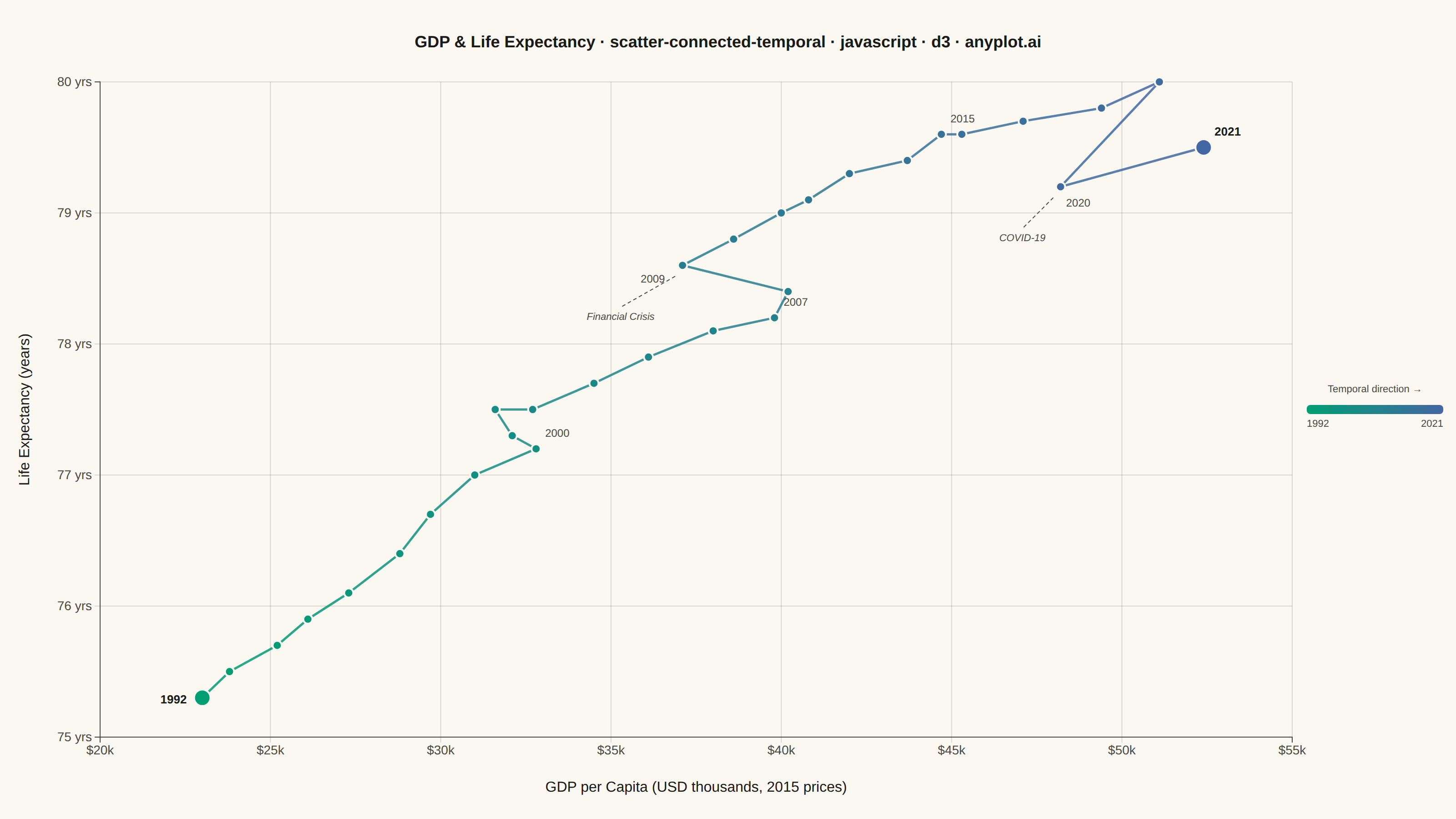
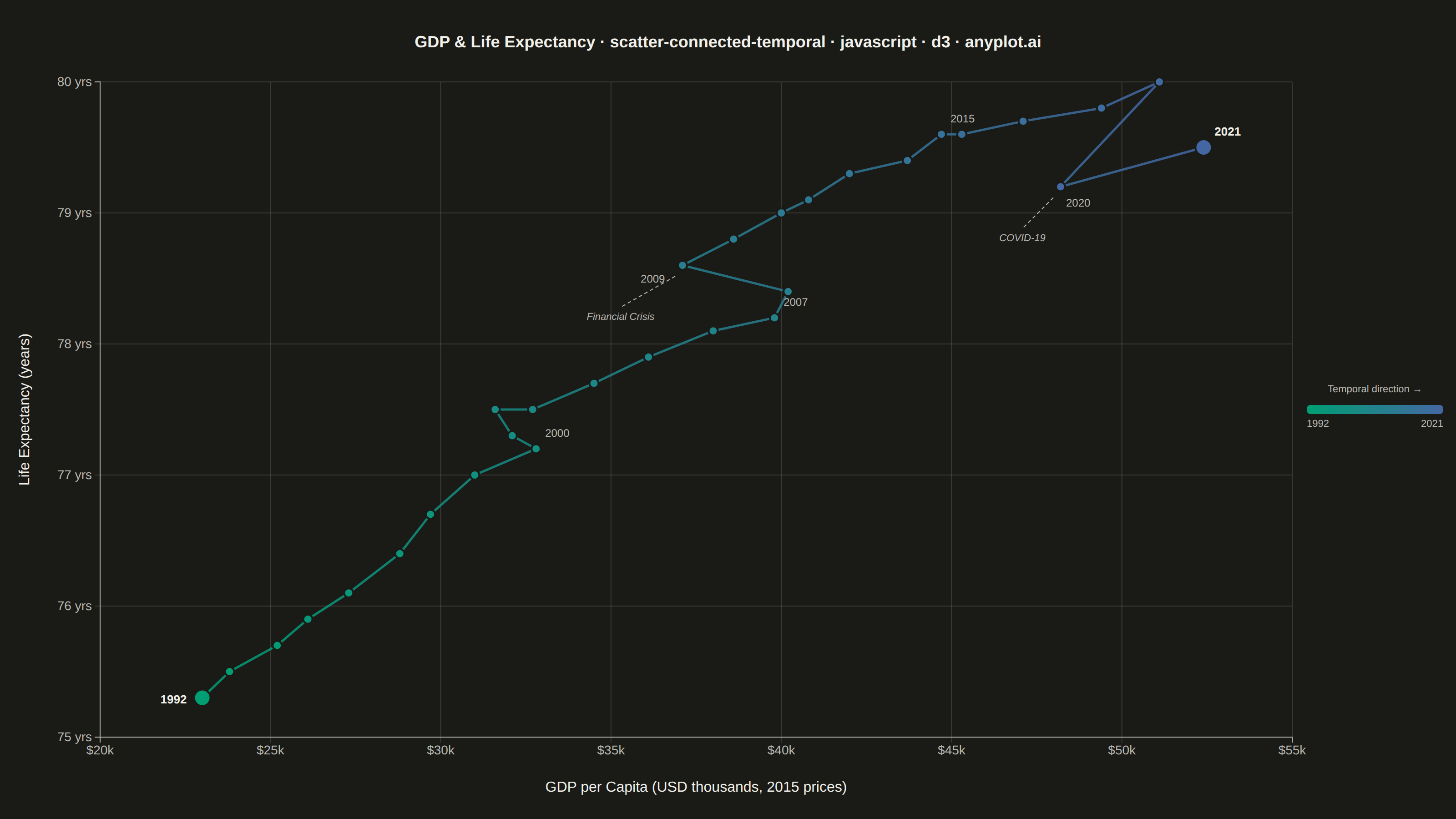
The same plot in 14 other libraries — JavaScript: Chart.js, Apache ECharts, Highcharts, MUI X Charts; Python: Altair, Bokeh, lets-plot, Matplotlib, Plotly, plotnine, Pygal, Seaborn; R: ggplot2; Julia: Makie.jl. Compare all 15 side by side: Connected Scatter Plot with Temporal Path in Python, R, Julia and JavaScript.
A scatter plot where data points are connected by lines in temporal order, revealing how two variables co-evolve over time. Unlike standard time series plots that show one variable against time, this plot encodes time as movement through 2D space, making cyclical patterns, regime changes, and directional trends visible. Popularized by the New York Times, it is a powerful tool for narrative data visualization.
// anyplot.ai
// scatter-connected-temporal: Connected Scatter Plot with Temporal Path
// Library: d3 7.9.0 | JavaScript 22.23.3
// Quality: 84/100 | Updated: 2026-10-08

const t = window.ANYPLOT_TOKENS;
const { width, height } = window.ANYPLOT_SIZE;
const margin = { top: 90, right: 180, bottom: 90, left: 110 };
const iw = width - margin.left - margin.right;
const ih = height - margin.top - margin.bottom;

// GDP per capita (thousands USD, 2015 prices) vs. Life Expectancy (years), 1992–2021
const data = [
  { year: 1992, gdp: 23.0, le: 75.3 }, { year: 1993, gdp: 23.8, le: 75.5 },
  { year: 1994, gdp: 25.2, le: 75.7 }, { year: 1995, gdp: 26.1, le: 75.9 },
  { year: 1996, gdp: 27.3, le: 76.1 }, { year: 1997, gdp: 28.8, le: 76.4 },
  { year: 1998, gdp: 29.7, le: 76.7 }, { year: 1999, gdp: 31.0, le: 77.0 },
  { year: 2000, gdp: 32.8, le: 77.2 }, { year: 2001, gdp: 32.1, le: 77.3 },
  { year: 2002, gdp: 31.6, le: 77.5 }, { year: 2003, gdp: 32.7, le: 77.5 },
  { year: 2004, gdp: 34.5, le: 77.7 }, { year: 2005, gdp: 36.1, le: 77.9 },
  { year: 2006, gdp: 38.0, le: 78.1 }, { year: 2007, gdp: 39.8, le: 78.2 },
  { year: 2008, gdp: 40.2, le: 78.4 }, { year: 2009, gdp: 37.1, le: 78.6 },
  { year: 2010, gdp: 38.6, le: 78.8 }, { year: 2011, gdp: 40.0, le: 79.0 },
  { year: 2012, gdp: 40.8, le: 79.1 }, { year: 2013, gdp: 42.0, le: 79.3 },
  { year: 2014, gdp: 43.7, le: 79.4 }, { year: 2015, gdp: 44.7, le: 79.6 },
  { year: 2016, gdp: 45.3, le: 79.6 }, { year: 2017, gdp: 47.1, le: 79.7 },
  { year: 2018, gdp: 49.4, le: 79.8 }, { year: 2019, gdp: 51.1, le: 80.0 },
  { year: 2020, gdp: 48.2, le: 79.2 }, { year: 2021, gdp: 52.4, le: 79.5 },
];

// SVG scaffold
const svg = d3.select("#container").append("svg").attr("width", width).attr("height", height);
const defs = svg.append("defs");

// Legend gradient (green → blue for the legend bar)
const legendGrad = defs.append("linearGradient")
  .attr("id", "temporal-legend-grad")
  .attr("x1", "0%").attr("x2", "100%");
legendGrad.append("stop").attr("offset", "0%").attr("stop-color", t.seq[0]);
legendGrad.append("stop").attr("offset", "100%").attr("stop-color", t.seq[1]);

const g = svg.append("g").attr("transform", `translate(${margin.left},${margin.top})`);

// Scales
const xScale = d3.scaleLinear().domain(d3.extent(data, d => d.gdp)).nice().range([0, iw]);
const yScale = d3.scaleLinear().domain(d3.extent(data, d => d.le)).nice().range([ih, 0]);

// Path-stroke gradient via gradientUnits="userSpaceOnUse" (idiomatic SVG/D3 technique)
// Projects color linearly from the 1992 start point to the 2021 end point in data space
const pathGrad = defs.append("linearGradient")
  .attr("id", "path-temporal-grad")
  .attr("gradientUnits", "userSpaceOnUse")
  .attr("x1", xScale(data[0].gdp))
  .attr("y1", yScale(data[0].le))
  .attr("x2", xScale(data[data.length - 1].gdp))
  .attr("y2", yScale(data[data.length - 1].le));
pathGrad.append("stop").attr("offset", "0%").attr("stop-color", t.seq[0]);
pathGrad.append("stop").attr("offset", "100%").attr("stop-color", t.seq[1]);

// Gridlines (both axes — subtle)
xScale.ticks(6).forEach(v => {
  g.append("line")
    .attr("x1", xScale(v)).attr("x2", xScale(v))
    .attr("y1", 0).attr("y2", ih)
    .attr("stroke", t.grid).attr("stroke-width", 1);
});
yScale.ticks(6).forEach(v => {
  g.append("line")
    .attr("x1", 0).attr("x2", iw)
    .attr("y1", yScale(v)).attr("y2", yScale(v))
    .attr("stroke", t.grid).attr("stroke-width", 1);
});

// Connecting path with userSpaceOnUse gradient stroke — single <path> element
const lineGen = d3.line()
  .x(d => xScale(d.gdp))
  .y(d => yScale(d.le));

g.append("path")
  .datum(data)
  .attr("d", lineGen)
  .attr("fill", "none")
  .attr("stroke", "url(#path-temporal-grad)")
  .attr("stroke-width", 2.5)
  .attr("stroke-opacity", 0.85);

// Temporal color interpolator (for marker fills, mirrors gradient)
const tempColor = frac => d3.interpolateRgb(t.seq[0], t.seq[1])(frac);

// Data point markers (larger endpoint circles for 1992 and 2021)
g.selectAll("circle").data(data).join("circle")
  .attr("cx", d => xScale(d.gdp))
  .attr("cy", d => yScale(d.le))
  .attr("r", (d, i) => (i === 0 || i === data.length - 1) ? 9 : 5)
  .attr("fill", (d, i) => tempColor(i / (data.length - 1)))
  .attr("stroke", t.pageBg)
  .attr("stroke-width", 2);

// Year labels at key economic moments
const labelConfig = [
  { year: 1992, dx: -46, dy: 6 },
  { year: 2000, dx: 10, dy: -13 },
  { year: 2007, dx: 10, dy: -13 },
  { year: 2009, dx: -46, dy: 19 },
  { year: 2015, dx: 10, dy: -13 },
  { year: 2020, dx: 6, dy: 22 },
  { year: 2021, dx: 12, dy: -13 },
];
data.forEach(d => {
  const cfg = labelConfig.find(c => c.year === d.year);
  if (!cfg) return;
  const isEndpoint = d.year === 1992 || d.year === 2021;
  g.append("text")
    .attr("x", xScale(d.gdp) + cfg.dx)
    .attr("y", yScale(d.le) + cfg.dy)
    .attr("fill", isEndpoint ? t.ink : t.inkSoft)
    .style("font-size", isEndpoint ? "13px" : "12px")
    .style("font-weight", isEndpoint ? "700" : "400")
    .text(d.year);
});

// Narrative event annotations with dashed leader lines
const d2009 = data.find(d => d.year === 2009);
const d2020 = data.find(d => d.year === 2020);

// Financial Crisis (2009) — leader line angling down-left, away from year label
const fc2009x = xScale(d2009.gdp) - 68;
const fc2009y = yScale(d2009.le) + 60;
g.append("line")
  .attr("x1", xScale(d2009.gdp) - 8).attr("y1", yScale(d2009.le) + 12)
  .attr("x2", fc2009x).attr("y2", fc2009y - 14)
  .attr("stroke", t.inkSoft).attr("stroke-width", 1).attr("stroke-dasharray", "4,3");
g.append("text")
  .attr("x", fc2009x).attr("y", fc2009y)
  .attr("text-anchor", "middle")
  .attr("fill", t.inkSoft).style("font-size", "13px").style("font-style", "italic")
  .text("Financial Crisis");

// COVID-19 (2020) — leader line going straight down, away from year label
const cv2020x = xScale(d2020.gdp) - 42;
const cv2020y = yScale(d2020.le) + 60;
g.append("line")
  .attr("x1", xScale(d2020.gdp) - 8).attr("y1", yScale(d2020.le) + 12)
  .attr("x2", cv2020x).attr("y2", cv2020y - 14)
  .attr("stroke", t.inkSoft).attr("stroke-width", 1).attr("stroke-dasharray", "4,3");
g.append("text")
  .attr("x", cv2020x).attr("y", cv2020y)
  .attr("text-anchor", "middle")
  .attr("fill", t.inkSoft).style("font-size", "13px").style("font-style", "italic")
  .text("COVID-19");

// Axes
const xAxis = g.append("g")
  .attr("transform", `translate(0,${ih})`)
  .call(d3.axisBottom(xScale).ticks(6).tickFormat(d => `$${d3.format(".0f")(d)}k`));
const yAxis = g.append("g")
  .call(d3.axisLeft(yScale).ticks(6).tickFormat(d => `${d3.format(".0f")(d)} yrs`));

[xAxis, yAxis].forEach(ax => {
  ax.selectAll("text").attr("fill", t.inkSoft).style("font-size", "14px");
  ax.selectAll("line").attr("stroke", t.grid);
  ax.select(".domain").attr("stroke", t.inkSoft);
});

// Axis labels
g.append("text")
  .attr("x", iw / 2).attr("y", ih + 60)
  .attr("text-anchor", "middle")
  .attr("fill", t.ink).style("font-size", "16px")
  .text("GDP per Capita (USD thousands, 2015 prices)");
g.append("text")
  .attr("transform", "rotate(-90)")
  .attr("x", -(ih / 2)).attr("y", -78)
  .attr("text-anchor", "middle")
  .attr("fill", t.ink).style("font-size", "16px")
  .text("Life Expectancy (years)");

// Temporal legend in the right margin — no overlap with data path
const lgW = 150, lgH = 10;
const lgX = iw + 16, lgY = ih / 2 - lgH / 2;
g.append("text")
  .attr("x", lgX + lgW / 2).attr("y", lgY - 14)
  .attr("text-anchor", "middle")
  .attr("fill", t.inkSoft).style("font-size", "13px")
  .text("Temporal direction  →");
g.append("rect")
  .attr("x", lgX).attr("y", lgY)
  .attr("width", lgW).attr("height", lgH)
  .attr("rx", 4)
  .attr("fill", "url(#temporal-legend-grad)");
g.append("text")
  .attr("x", lgX).attr("y", lgY + lgH + 14)
  .attr("fill", t.inkSoft).style("font-size", "13px")
  .text("1992");
g.append("text")
  .attr("x", lgX + lgW).attr("y", lgY + lgH + 14)
  .attr("text-anchor", "end")
  .attr("fill", t.inkSoft).style("font-size", "13px")
  .text("2021");

// Title
const title = "GDP & Life Expectancy · scatter-connected-temporal · javascript · d3 · anyplot.ai";
const titleFontSize = Math.max(13, Math.round(22 * 67 / title.length));
svg.append("text")
  .attr("x", width / 2).attr("y", 52)
  .attr("text-anchor", "middle")
  .attr("fill", t.ink)
  .style("font-size", `${titleFontSize}px`)
  .style("font-weight", "600")
  .text(title);
Runnable source as JSON, for any HTTP client: https://api.anyplot.ai/specs/scatter-connected-temporal/d3/code. Any spec id and library id listed in llms-full.txt fit the same URL shape; every URL below is complete and callable.
{
  "spec_id": "scatter-connected-temporal",
  "language": "javascript",
  "library": "d3",
  "page": "https://anyplot.ai/scatter-connected-temporal/javascript/d3",
  "hub": "https://anyplot.ai/scatter-connected-temporal",
  "code_json": "https://api.anyplot.ai/specs/scatter-connected-temporal/d3/code",
  "spec_json": "https://api.anyplot.ai/specs/scatter-connected-temporal",
  "render_light_png": "https://storage.googleapis.com/anyplot-images/plots/scatter-connected-temporal/javascript/d3/plot-light.png",
  "render_dark_png": "https://storage.googleapis.com/anyplot-images/plots/scatter-connected-temporal/javascript/d3/plot-dark.png",
  "interactive_light_html": "https://storage.googleapis.com/anyplot-images/plots/scatter-connected-temporal/javascript/d3/plot-light.html",
  "interactive_dark_html": "https://storage.googleapis.com/anyplot-images/plots/scatter-connected-temporal/javascript/d3/plot-dark.html",
  "quality_score": 84.0,
  "license": "MIT",
  "guide": "https://anyplot.ai/llms.txt"
}
Part of Connected Scatter Plot with Temporal Path on anyplot.ai.