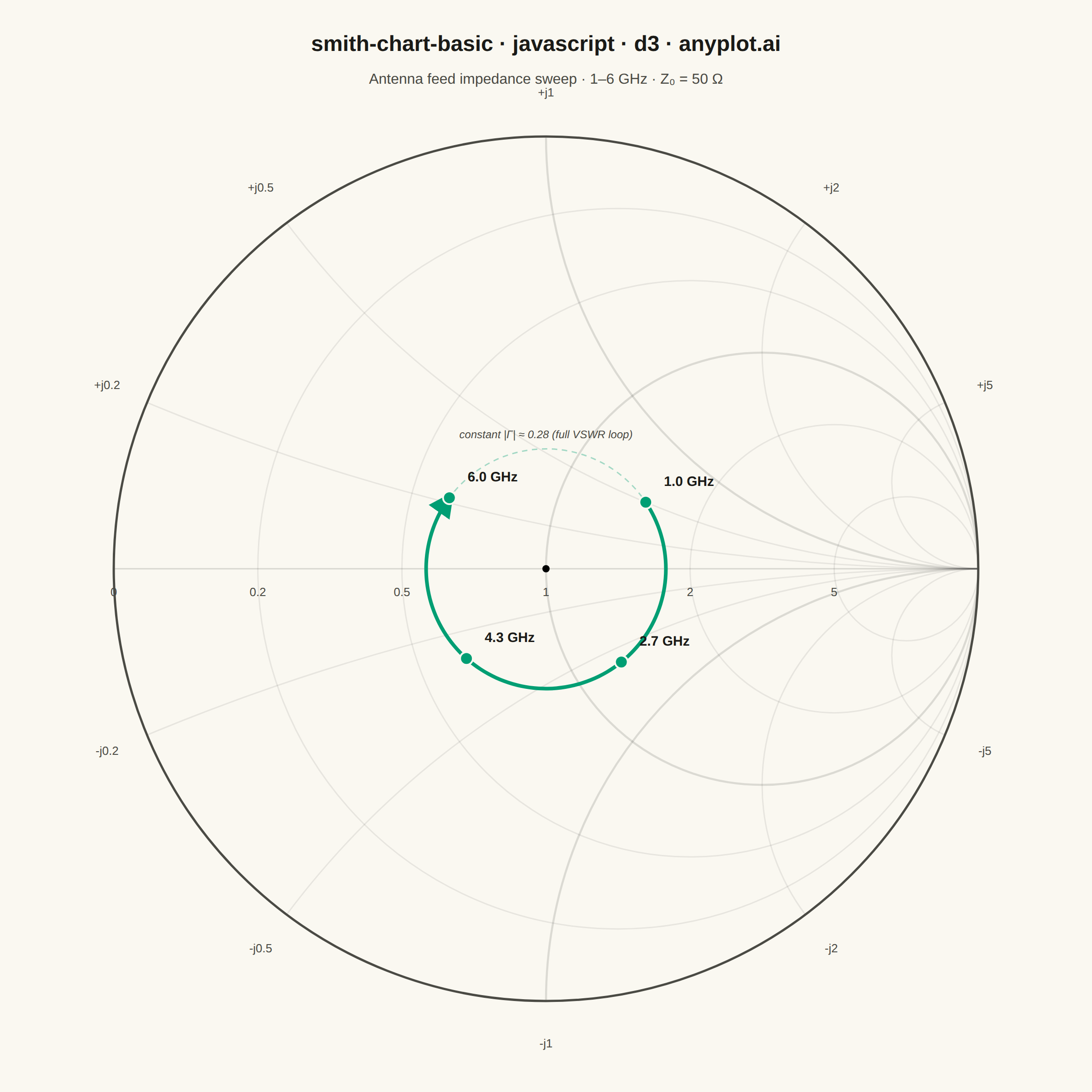
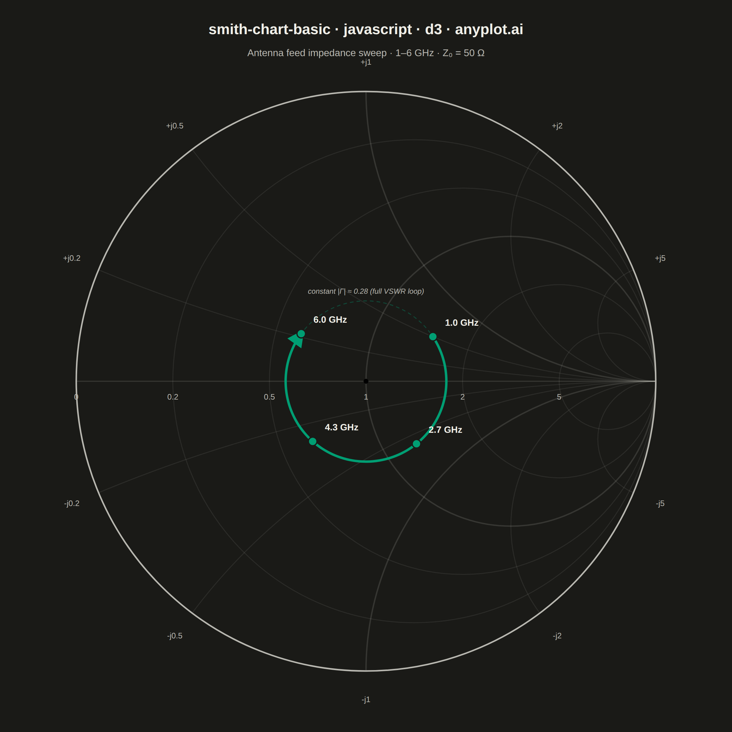
The same plot in 14 other libraries — JavaScript: Chart.js, Apache ECharts, Highcharts, MUI X Charts; Python: Altair, Bokeh, lets-plot, Matplotlib, Plotly, plotnine, Pygal, Seaborn; R: ggplot2; Julia: Makie.jl. Compare all 15 side by side: Smith Chart for RF/Impedance in Python, R, Julia and JavaScript.
A Smith chart is a specialized circular diagram used in RF engineering to display complex impedance and reflection coefficients on a normalized polar grid. The chart features constant resistance circles (centered along the horizontal axis) and constant reactance arcs (curving from the right edge), enabling engineers to visualize impedance matching, transmission line behavior, and antenna characteristics. It reveals relationships between impedance, admittance, and reflection coefficient that would be difficult to interpret in Cartesian coordinates.
// anyplot.ai
// smith-chart-basic: Smith Chart for RF/Impedance
// Library: d3 7.9.0 | JavaScript 22.23.2
// Quality: 93/100 | Created: 2026-09-02

//# anyplot-orientation: square
const t = window.ANYPLOT_TOKENS;
const { width, height } = window.ANYPLOT_SIZE;

// Complex-number helpers — the browser has no built-in complex type
const cSub = (a, b) => ({ re: a.re - b.re, im: a.im - b.im });
const cDiv = (a, b) => {
  const denom = b.re * b.re + b.im * b.im;
  return { re: (a.re * b.re + a.im * b.im) / denom, im: (a.im * b.re - a.re * b.im) / denom };
};

// Antenna feed-point impedance seen at the input of a lossless line as the
// sweep frequency changes the line's electrical length: |gamma| stays fixed
// at the load's magnitude while its phase rotates, tracing the classic
// constant-VSWR arc that a network analyzer records during S11 sweeps.
const z0 = 50; // Reference impedance (ohms)
const zLoad = { re: 75, im: 25 }; // Mismatched antenna feed, ohms
const gammaLoad = cDiv(cSub(zLoad, { re: z0, im: 0 }), { re: zLoad.re + z0, im: zLoad.im });
const gammaLoadMag = Math.hypot(gammaLoad.re, gammaLoad.im);
const gammaLoadPhase = Math.atan2(gammaLoad.im, gammaLoad.re);

const pointCount = 60;
const freqStartHz = 1e9;
const freqEndHz = 6e9;
const sweepDegrees = 250; // total electrical-length rotation across the band

const impedanceData = d3.range(pointCount).map((i) => {
  const frac = i / (pointCount - 1);
  const frequency = freqStartHz + frac * (freqEndHz - freqStartHz);
  const phase = gammaLoadPhase - frac * (sweepDegrees * Math.PI) / 180;
  const gamma = { re: gammaLoadMag * Math.cos(phase), im: gammaLoadMag * Math.sin(phase) };
  const z = cDiv({ re: z0 * (1 + gamma.re), im: z0 * gamma.im }, cSub({ re: 1, im: 0 }, gamma));
  return { frequency, z_real: z.re, z_imag: z.im };
});

// Normalize to Z/Z0 and derive the reflection coefficient for plotting
const locus = impedanceData.map((d) => {
  const zn = { re: d.z_real / z0, im: d.z_imag / z0 };
  return cDiv(cSub(zn, { re: 1, im: 0 }), { re: zn.re + 1, im: zn.im });
});

// Layout — the chart itself is circular, so it earns the square canvas
const margin = { top: 150, right: 100, bottom: 100, left: 100 };
const plotSize = Math.min(width - margin.left - margin.right, height - margin.top - margin.bottom);
const radius = plotSize / 2;
const cx = width / 2;
const cy = margin.top + plotSize / 2;
const toPixel = (re, im) => [cx + re * radius, cy - im * radius];
const boundaryPoint = (x) => {
  const denom = x * x + 1;
  return [(x * x - 1) / denom, (2 * x) / denom];
};

// SVG mount
const svg = d3.select("#container").append("svg").attr("width", width).attr("height", height);
const defs = svg.append("defs");
defs.append("clipPath").attr("id", "smith-boundary")
  .append("circle").attr("cx", cx).attr("cy", cy).attr("r", radius);
defs.append("marker")
  .attr("id", "locus-arrow")
  .attr("viewBox", "0 0 10 10")
  .attr("refX", 7).attr("refY", 5)
  .attr("markerWidth", 7).attr("markerHeight", 7)
  .attr("orient", "auto-start-reverse")
  .append("path")
  .attr("d", "M0,0 L10,5 L0,10 Z")
  .attr("fill", t.palette[0]);

// Grid — constant-resistance circles and constant-reactance arcs, clipped to
// the unit circle since only the arcs' interior segments are meaningful.
// The r=1 / x=1 circles are the Smith chart's "major" reference curves, so
// they render slightly bolder than the rest to establish visual hierarchy.
const grid = svg.append("g").attr("clip-path", "url(#smith-boundary)");
const resistanceValues = [0.2, 0.5, 1, 2, 5];
const reactanceValues = [0.2, 0.5, 1, 2, 5];
const reactanceCircles = reactanceValues.flatMap((x) => [1, -1].map((sign) => ({ x, sign })));

grid.append("line")
  .attr("x1", cx - radius).attr("y1", cy).attr("x2", cx + radius).attr("y2", cy)
  .attr("stroke", t.grid).attr("stroke-width", 1.5);

grid.selectAll(".resistance-circle")
  .data(resistanceValues)
  .join("circle")
  .attr("class", "resistance-circle")
  .attr("cx", (r) => cx + (r / (r + 1)) * radius)
  .attr("cy", cy)
  .attr("r", (r) => radius / (r + 1))
  .attr("fill", "none")
  .attr("stroke", t.grid)
  .attr("stroke-width", (r) => (r === 1 ? 2.25 : 1.5))
  .attr("opacity", (r) => (r === 1 ? 0.9 : 0.55));

grid.selectAll(".reactance-circle")
  .data(reactanceCircles)
  .join("circle")
  .attr("class", "reactance-circle")
  .attr("cx", cx + radius)
  .attr("cy", (d) => cy - radius / (d.sign * d.x))
  .attr("r", (d) => Math.abs(radius / (d.sign * d.x)))
  .attr("fill", "none")
  .attr("stroke", t.grid)
  .attr("stroke-width", (d) => (d.x === 1 ? 2.25 : 1.5))
  .attr("opacity", (d) => (d.x === 1 ? 0.9 : 0.55));

// Optional constant-VSWR circle — the load's |gamma| stays fixed as a lossless
// line's electrical length rotates its phase, so the swept locus below is one
// arc of this full circle. Dashed and low-opacity to read as context, not data.
const vswrRadius = gammaLoadMag * radius;
svg.append("circle")
  .attr("cx", cx).attr("cy", cy).attr("r", vswrRadius)
  .attr("fill", "none").attr("stroke", t.palette[0])
  .attr("stroke-width", 1.5).attr("stroke-dasharray", "6 5")
  .attr("opacity", 0.35);
svg.append("text")
  .attr("x", cx).attr("y", cy - vswrRadius - 12)
  .attr("text-anchor", "middle")
  .attr("fill", t.inkSoft).style("font-size", "12px").style("font-style", "italic")
  .text(`constant |Γ| ≈ ${gammaLoadMag.toFixed(2)} (full VSWR loop)`);

// Boundary circle |gamma| = 1 — total reflection, drawn crisp on top of the grid
svg.append("circle")
  .attr("cx", cx).attr("cy", cy).attr("r", radius)
  .attr("fill", "none").attr("stroke", t.inkSoft).attr("stroke-width", 2.5);

// Matched-condition marker at the chart center (Z = Z0, gamma = 0)
svg.append("circle").attr("cx", cx).attr("cy", cy).attr("r", 4).attr("fill", t.muted);

// Resistance-circle labels along the real axis, offset below their tangent
// point with extra padding so the r=0 label clears the boundary circle.
svg.selectAll(".resistance-label")
  .data(resistanceValues.concat([0]))
  .join("text")
  .attr("class", "resistance-label")
  .attr("x", (r) => toPixel((r - 1) / (r + 1), 0)[0])
  .attr("y", (r) => toPixel((r - 1) / (r + 1), 0)[1] + 30)
  .attr("text-anchor", "middle")
  .attr("fill", t.inkSoft).style("font-size", "13px")
  .text((r) => r);

// Reactance-arc labels just outside the boundary, at each arc's exit point
const reactanceLabelData = reactanceCircles.map((d) => {
  const [gx, gy] = boundaryPoint(d.sign * d.x);
  const angle = Math.atan2(gy, gx);
  return { ...d, lx: cx + Math.cos(angle) * radius * 1.1, ly: cy - Math.sin(angle) * radius * 1.1 };
});

svg.selectAll(".reactance-label")
  .data(reactanceLabelData)
  .join("text")
  .attr("class", "reactance-label")
  .attr("x", (d) => d.lx).attr("y", (d) => d.ly)
  .attr("text-anchor", "middle").attr("dominant-baseline", "middle")
  .attr("fill", t.inkSoft).style("font-size", "13px")
  .text((d) => `${d.sign > 0 ? "+" : "-"}j${d.x}`);

// Impedance locus — the frequency-swept trajectory across the reflection
// plane, with an arrowhead marking the sweep direction (low to high frequency)
const lineGen = d3.line()
  .x((d) => toPixel(d.re, d.im)[0])
  .y((d) => toPixel(d.re, d.im)[1])
  .curve(d3.curveCatmullRom.alpha(0.5));

svg.append("path")
  .datum(locus)
  .attr("fill", "none")
  .attr("stroke", t.palette[0])
  .attr("stroke-width", 4)
  .attr("stroke-linejoin", "round")
  .attr("marker-end", "url(#locus-arrow)")
  .attr("d", lineGen);

// Frequency markers at the sweep endpoints and two intermediate points
const markerIndices = [0, Math.round((pointCount - 1) / 3), Math.round((2 * (pointCount - 1)) / 3), pointCount - 1];
const markerData = markerIndices.map((i) => ({ ...locus[i], frequency: impedanceData[i].frequency }));

const markers = svg.selectAll(".freq-marker")
  .data(markerData)
  .join("g")
  .attr("class", "freq-marker");

markers.append("circle")
  .attr("cx", (d) => toPixel(d.re, d.im)[0])
  .attr("cy", (d) => toPixel(d.re, d.im)[1])
  .attr("r", 7)
  .attr("fill", t.palette[0]).attr("stroke", t.pageBg).attr("stroke-width", 2);

markers.append("text")
  .attr("x", (d) => toPixel(d.re, d.im)[0] + 20)
  .attr("y", (d) => toPixel(d.re, d.im)[1] - 18)
  .attr("fill", t.ink).style("font-size", "15px").style("font-weight", "600")
  .text((d) => `${(d.frequency / 1e9).toFixed(1)} GHz`);

// Title + subtitle
const title = "smith-chart-basic · javascript · d3 · anyplot.ai";
svg.append("text")
  .attr("x", width / 2).attr("y", 56)
  .attr("text-anchor", "middle")
  .attr("fill", t.ink).style("font-size", "24px").style("font-weight", "600")
  .text(title);

svg.append("text")
  .attr("x", width / 2).attr("y", 92)
  .attr("text-anchor", "middle")
  .attr("fill", t.inkSoft).style("font-size", "16px")
  .text("Antenna feed impedance sweep · 1–6 GHz · Z₀ = 50 Ω");
Runnable source as JSON, for any HTTP client: https://api.anyplot.ai/specs/smith-chart-basic/d3/code. Any spec id and library id listed in llms-full.txt fit the same URL shape; every URL below is complete and callable.
{
  "spec_id": "smith-chart-basic",
  "language": "javascript",
  "library": "d3",
  "page": "https://anyplot.ai/smith-chart-basic/javascript/d3",
  "hub": "https://anyplot.ai/smith-chart-basic",
  "code_json": "https://api.anyplot.ai/specs/smith-chart-basic/d3/code",
  "spec_json": "https://api.anyplot.ai/specs/smith-chart-basic",
  "render_light_png": "https://storage.googleapis.com/anyplot-images/plots/smith-chart-basic/javascript/d3/plot-light.png",
  "render_dark_png": "https://storage.googleapis.com/anyplot-images/plots/smith-chart-basic/javascript/d3/plot-dark.png",
  "interactive_light_html": "https://storage.googleapis.com/anyplot-images/plots/smith-chart-basic/javascript/d3/plot-light.html",
  "interactive_dark_html": "https://storage.googleapis.com/anyplot-images/plots/smith-chart-basic/javascript/d3/plot-dark.html",
  "quality_score": 93.0,
  "license": "MIT",
  "guide": "https://anyplot.ai/llms.txt"
}
Part of Smith Chart for RF/Impedance on anyplot.ai.