The same plot in 14 other libraries — Python: Altair, Bokeh, lets-plot, Matplotlib, Plotly, plotnine, Pygal, Seaborn; Julia: Makie.jl; JavaScript: Chart.js, D3.js, Apache ECharts, Highcharts, MUI X Charts. Compare all 15 side by side: Smith Chart for RF/Impedance in Python, R, Julia and JavaScript.
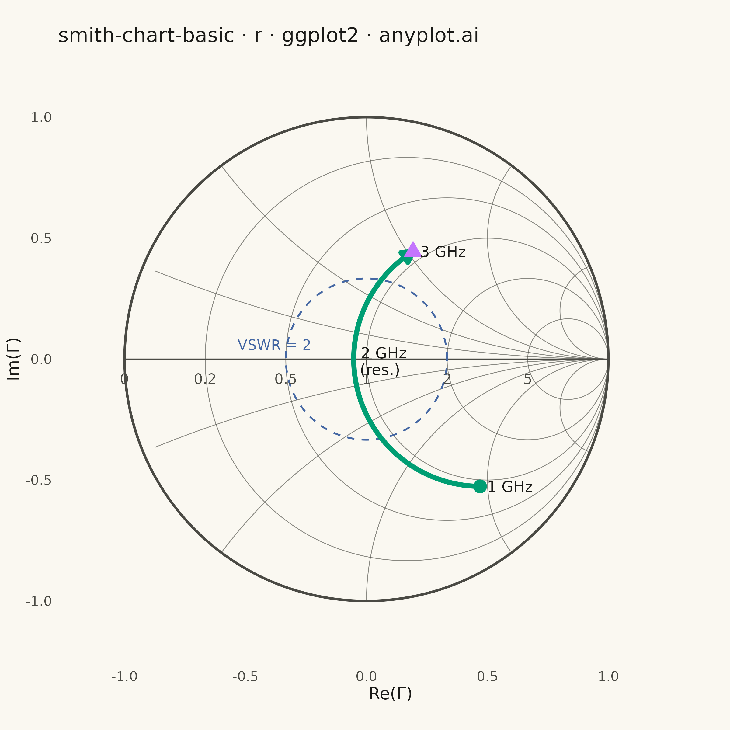
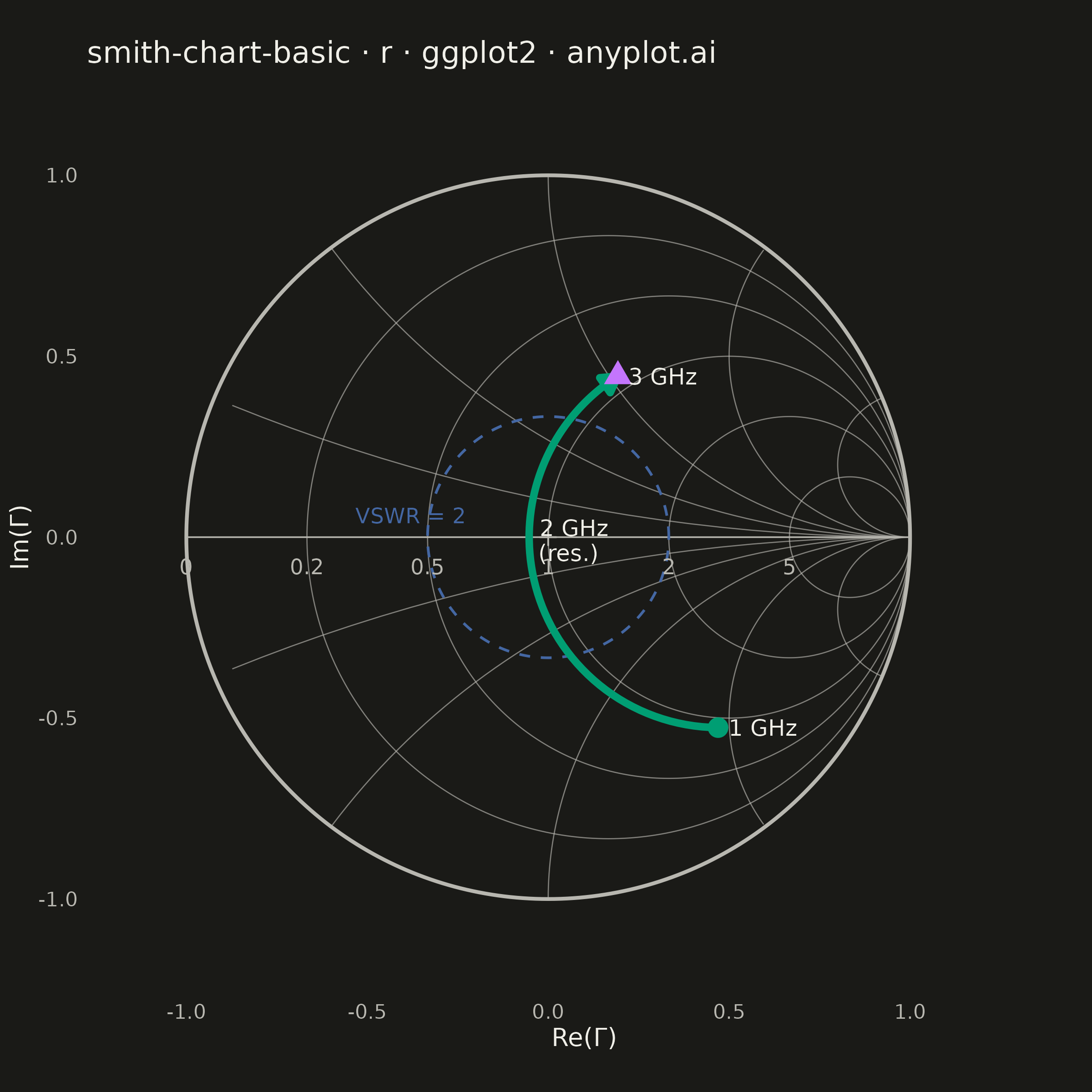
A Smith chart is a specialized circular diagram used in RF engineering to display complex impedance and reflection coefficients on a normalized polar grid. The chart features constant resistance circles (centered along the horizontal axis) and constant reactance arcs (curving from the right edge), enabling engineers to visualize impedance matching, transmission line behavior, and antenna characteristics. It reveals relationships between impedance, admittance, and reflection coefficient that would be difficult to interpret in Cartesian coordinates.
#' anyplot.ai
#' smith-chart-basic: Smith Chart for RF/Impedance
#' Library: ggplot2 3.5.1 | R 4.4.1
#' Quality: 89/100 | Created: 2026-05-20

library(ggplot2)
library(ragg)

# --- Theme tokens -----------------------------------------------------------
THEME       <- Sys.getenv("ANYPLOT_THEME", "light")
PAGE_BG     <- if (THEME == "light") "#FAF8F1" else "#1A1A17"
INK         <- if (THEME == "light") "#1A1A17" else "#F0EFE8"
INK_SOFT    <- if (THEME == "light") "#4A4A44" else "#B8B7B0"
IMPRINT   <- c("#009E73", "#C475FD", "#4467A3", "#BD8233",
                 "#AE3030", "#2ABCCD", "#954477")

# --- Smith chart grid -------------------------------------------------------
theta <- seq(0, 2 * pi, length.out = 361)

# Outer unit circle (|Gamma| = 1 boundary)
outer_circle <- data.frame(x = cos(theta), y = sin(theta))

# Constant resistance circles: r/(1+r) center, 1/(1+r) radius
r_vals <- c(0, 0.2, 0.5, 1, 2, 5)
r_circles <- do.call(rbind, lapply(r_vals, function(r) {
  cx  <- r / (1 + r)
  rad <- 1 / (1 + r)
  data.frame(
    x   = cx + rad * cos(theta),
    y   = rad * sin(theta),
    grp = paste0("r", r)
  )
}))

# Constant reactance arcs: center (1, 1/x), radius 1/|x|, clipped to unit disc
x_vals <- c(0.2, 0.5, 1, 2, 5)
x_arcs <- do.call(rbind, lapply(c(x_vals, -x_vals), function(x) {
  cy  <- 1 / x
  rad <- abs(1 / x)
  pts_x <- 1 + rad * cos(theta)
  pts_y <- cy  + rad * sin(theta)
  inside <- (pts_x^2 + pts_y^2) <= 1.001
  if (sum(inside) < 3) return(NULL)
  data.frame(x = pts_x[inside], y = pts_y[inside], grp = paste0("x", x))
}))

# VSWR = 2 reference circle (|Gamma| = 1/3)
vswr_circle <- data.frame(
  x = (1 / 3) * cos(theta),
  y = (1 / 3) * sin(theta)
)

# --- Impedance locus: RLC antenna resonant near 2 GHz ----------------------
set.seed(42)
Z0        <- 50
freqs_ghz <- seq(1, 3, length.out = 80)
omega     <- 2 * pi * freqs_ghz * 1e9

R_ant <- 45
L_ant <- 5e-9
C_ant <- 1 / ((2 * pi * 2e9)^2 * L_ant)   # resonance exactly at 2 GHz

zr <- R_ant / Z0
zx <- (omega * L_ant - 1 / (omega * C_ant)) / Z0

# Reflection coefficient Gamma = (z - 1) / (z + 1)
denom    <- (zr + 1)^2 + zx^2
gamma_re <- ((zr - 1) * (zr + 1) + zx^2) / denom
gamma_im <- 2 * zx / denom

locus <- data.frame(gre = gamma_re, gim = gamma_im, freq = freqs_ghz)

# Labels at 1 GHz, 2 GHz, 3 GHz
label_freqs <- c(1, 2, 3)
label_idx   <- sapply(label_freqs, function(f) which.min(abs(locus$freq - f)))
label_pts   <- locus[label_idx, ]
label_pts$lbl <- c("1 GHz", "2 GHz\n(res.)", "3 GHz")

# Directional arrow at 3 GHz end to show sweep direction
n_loc <- nrow(locus)
dx    <- locus$gre[n_loc] - locus$gre[n_loc - 5]
dy    <- locus$gim[n_loc] - locus$gim[n_loc - 5]
norm  <- sqrt(dx^2 + dy^2)
arr_len <- 0.055
arr_x0  <- locus$gre[n_loc] - (dx / norm) * arr_len
arr_y0  <- locus$gim[n_loc] - (dy / norm) * arr_len

# --- Plot -------------------------------------------------------------------
p <- ggplot() +
  # Grid: outer circle
  geom_path(data = outer_circle, aes(x = x, y = y),
            color = INK_SOFT, linewidth = 0.7) +
  # Grid: constant-r circles
  geom_path(data = r_circles, aes(x = x, y = y, group = grp),
            color = INK_SOFT, linewidth = 0.22, alpha = 0.65) +
  # Grid: constant-x arcs
  geom_path(data = x_arcs, aes(x = x, y = y, group = grp),
            color = INK_SOFT, linewidth = 0.22, alpha = 0.65) +
  # Real axis
  geom_segment(aes(x = -1, xend = 1, y = 0, yend = 0),
               color = INK_SOFT, linewidth = 0.3) +
  # VSWR = 2 reference circle
  geom_path(data = vswr_circle, aes(x = x, y = y),
            color = IMPRINT[3], linewidth = 0.5, linetype = "dashed") +
  annotate("text", x = -0.38, y = 0.06,
           label = "VSWR = 2", size = 3.0, color = IMPRINT[3]) +
  # Matched-load centre marker
  geom_point(aes(x = 0, y = 0),
             color = INK_SOFT, size = 1.8, shape = 3) +
  # Impedance locus
  geom_path(data = locus, aes(x = gre, y = gim),
            color = IMPRINT[1], linewidth = 1.4) +
  # Directional arrow at 3 GHz end showing sweep direction
  annotate("segment",
           x = arr_x0, xend = locus$gre[n_loc],
           y = arr_y0, yend = locus$gim[n_loc],
           color = IMPRINT[1], linewidth = 1.4,
           arrow = arrow(length = unit(0.1, "inches"), type = "closed")) +
  # Start (1 GHz) and end (3 GHz) markers
  geom_point(data = locus[1, ], aes(x = gre, y = gim),
             color = IMPRINT[1], size = 3.5, shape = 16) +
  geom_point(data = locus[nrow(locus), ], aes(x = gre, y = gim),
             color = IMPRINT[2], size = 3.5, shape = 17) +
  # Frequency labels
  geom_text(data = label_pts, aes(x = gre, y = gim, label = lbl),
            color = INK, size = 3.2, hjust = -0.15, lineheight = 0.9) +
  # Resistance value labels along real axis
  annotate("text",
           x = (r_vals - 1) / (r_vals + 1),
           y = -0.06,
           label = as.character(r_vals),
           size = 3.0, color = INK_SOFT, vjust = 1) +
  coord_fixed(xlim = c(-1.15, 1.35), ylim = c(-1.15, 1.15)) +
  labs(
    title = "smith-chart-basic · r · ggplot2 · anyplot.ai",
    x     = "Re(Γ)",
    y     = "Im(Γ)"
  ) +
  theme_minimal(base_size = 8) +
  theme(
    plot.background  = element_rect(fill = PAGE_BG, color = PAGE_BG),
    panel.background = element_rect(fill = PAGE_BG, color = NA),
    panel.grid.major = element_blank(),
    panel.grid.minor = element_blank(),
    panel.border     = element_blank(),
    axis.title       = element_text(color = INK,      size = 10),
    axis.text        = element_text(color = INK_SOFT, size = 8),
    plot.title       = element_text(color = INK,      size = 12),
    axis.line        = element_blank()
  )

# --- Save -------------------------------------------------------------------
ggsave(
  filename = sprintf("plot-%s.png", THEME),
  plot     = p,
  device   = ragg::agg_png,
  width    = 6,
  height   = 6,
  units    = "in",
  dpi      = 400
)
Runnable source as JSON, for any HTTP client: https://api.anyplot.ai/specs/smith-chart-basic/ggplot2/code. Any spec id and library id listed in llms-full.txt fit the same URL shape; every URL below is complete and callable.
{
  "spec_id": "smith-chart-basic",
  "language": "r",
  "library": "ggplot2",
  "page": "https://anyplot.ai/smith-chart-basic/r/ggplot2",
  "hub": "https://anyplot.ai/smith-chart-basic",
  "code_json": "https://api.anyplot.ai/specs/smith-chart-basic/ggplot2/code",
  "spec_json": "https://api.anyplot.ai/specs/smith-chart-basic",
  "render_light_png": "https://storage.googleapis.com/anyplot-images/plots/smith-chart-basic/r/ggplot2/plot-light.png",
  "render_dark_png": "https://storage.googleapis.com/anyplot-images/plots/smith-chart-basic/r/ggplot2/plot-dark.png",
  "quality_score": 89.0,
  "license": "MIT",
  "guide": "https://anyplot.ai/llms.txt"
}
Part of Smith Chart for RF/Impedance on anyplot.ai.