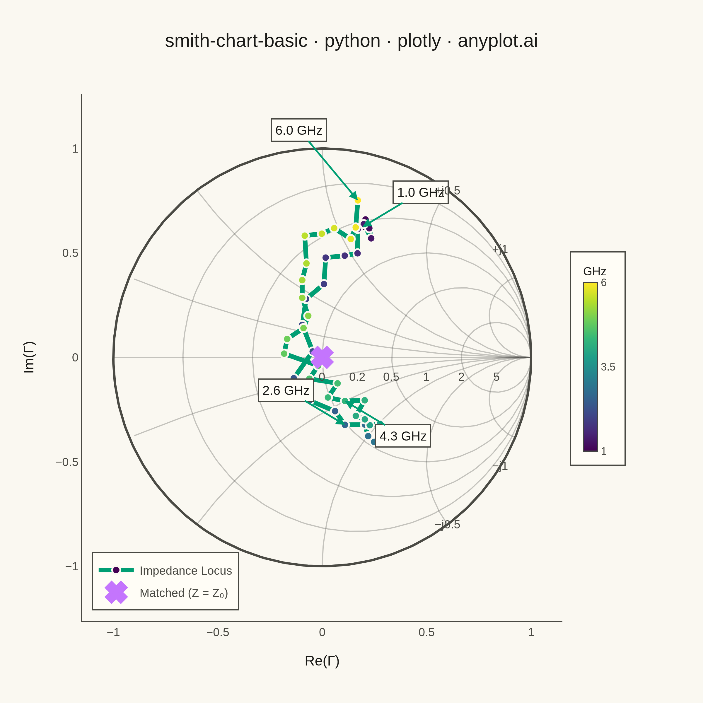
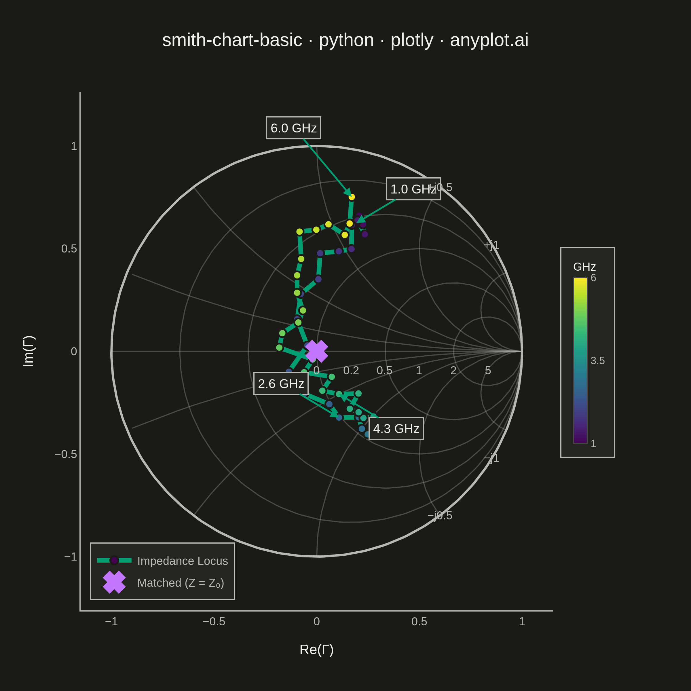
A Smith chart is a specialized circular diagram used in RF engineering to display complex impedance and reflection coefficients on a normalized polar grid. The chart features constant resistance circles (centered along the horizontal axis) and constant reactance arcs (curving from the right edge), enabling engineers to visualize impedance matching, transmission line behavior, and antenna characteristics. It reveals relationships between impedance, admittance, and reflection coefficient that would be difficult to interpret in Cartesian coordinates.
""" anyplot.ai
smith-chart-basic: Smith Chart for RF/Impedance
Library: plotly 6.7.0 | Python 3.13.13
Quality: 85/100 | Updated: 2026-05-20
"""

import os

import numpy as np
import plotly.graph_objects as go


THEME = os.getenv("ANYPLOT_THEME", "light")
PAGE_BG = "#FAF8F1" if THEME == "light" else "#1A1A17"
ELEVATED_BG = "#FFFDF6" if THEME == "light" else "#242420"
INK = "#1A1A17" if THEME == "light" else "#F0EFE8"
INK_SOFT = "#4A4A44" if THEME == "light" else "#B8B7B0"

BRAND = "#009E73"  # Okabe-Ito position 1 — impedance locus
ACCENT = "#C475FD"  # Okabe-Ito position 2 — matched condition marker

# Smith chart grid color (slightly stronger than RULE for chart structure)
SMITH_GRID = "rgba(74,74,68,0.30)" if THEME == "light" else "rgba(184,183,176,0.30)"

# Reference impedance
Z0 = 50  # ohms

# Generate sample impedance data (antenna-like frequency sweep, 1–6 GHz)
np.random.seed(42)
freq = np.linspace(1e9, 6e9, 50)

# Simulate realistic antenna impedance trajectory:
# starting inductive, sweeping through resonance to capacitive
t = np.linspace(0, 2 * np.pi, 50)
z_real = 25 + 40 * np.sin(t / 2) ** 2 + 5 * np.random.randn(50)
z_imag = 60 * np.cos(t) + 10 * np.sin(2 * t)

# Normalize impedance and calculate reflection coefficient (Γ)
z_norm = (z_real + 1j * z_imag) / Z0
gamma = (z_norm - 1) / (z_norm + 1)
gamma_real = gamma.real
gamma_imag = gamma.imag

fig = go.Figure()

# Smith chart grid — constant resistance circles
r_values = [0, 0.2, 0.5, 1, 2, 5]
theta_grid = np.linspace(0, 2 * np.pi, 200)

for r in r_values:
    center_x = r / (r + 1)
    radius = 1 / (r + 1)
    circle_x = center_x + radius * np.cos(theta_grid)
    circle_y = radius * np.sin(theta_grid)
    mask = circle_x**2 + circle_y**2 <= 1.01
    fig.add_trace(
        go.Scatter(
            x=np.where(mask, circle_x, np.nan),
            y=np.where(mask, circle_y, np.nan),
            mode="lines",
            line=dict(color=SMITH_GRID, width=1),
            hoverinfo="skip",
            showlegend=False,
        )
    )

# Smith chart grid — constant reactance arcs (positive and negative)
x_values = [0.2, 0.5, 1, 2, 5]
arc_theta = np.linspace(-np.pi, np.pi, 400)

for x in x_values:
    center_y = 1 / x
    radius = 1 / x
    arc_x = 1 + radius * np.cos(arc_theta)
    arc_y = center_y + radius * np.sin(arc_theta)
    mask = (arc_x**2 + arc_y**2 <= 1.01) & (arc_x >= -1)
    arc_x_clipped = np.where(mask, arc_x, np.nan)
    arc_y_clipped = np.where(mask, arc_y, np.nan)
    for sign in (1, -1):
        fig.add_trace(
            go.Scatter(
                x=arc_x_clipped,
                y=sign * arc_y_clipped,
                mode="lines",
                line=dict(color=SMITH_GRID, width=1),
                hoverinfo="skip",
                showlegend=False,
            )
        )

# Real axis
fig.add_trace(
    go.Scatter(
        x=[-1, 1], y=[0, 0], mode="lines", line=dict(color=SMITH_GRID, width=1), hoverinfo="skip", showlegend=False
    )
)

# Unit circle boundary (|Γ| = 1)
boundary_theta = np.linspace(0, 2 * np.pi, 300)
fig.add_trace(
    go.Scatter(
        x=np.cos(boundary_theta),
        y=np.sin(boundary_theta),
        mode="lines",
        line=dict(color=INK_SOFT, width=2),
        hoverinfo="skip",
        showlegend=False,
    )
)

# Impedance locus
freq_ghz = freq / 1e9
hover_text = [f"{f:.2f} GHz<br>Z = {z_real[i]:.1f} + j{z_imag[i]:.1f} Ω" for i, f in enumerate(freq_ghz)]
freq_normalized = np.linspace(0, 1, len(freq))
fig.add_trace(
    go.Scatter(
        x=gamma_real,
        y=gamma_imag,
        mode="lines+markers",
        line=dict(color=BRAND, width=4.0),
        marker=dict(
            size=7,
            color=freq_normalized,
            colorscale="viridis",
            showscale=True,
            colorbar=dict(
                title=dict(text="GHz", font=dict(size=10, color=INK), side="top"),
                tickvals=[0, 0.5, 1],
                ticktext=["1", "3.5", "6"],
                len=0.4,
                thickness=12,
                x=1.02,
                tickfont=dict(size=9, color=INK_SOFT),
                bgcolor=ELEVATED_BG,
                bordercolor=INK_SOFT,
                borderwidth=1,
            ),
            line=dict(color=PAGE_BG, width=1.5),
        ),
        name="Impedance Locus",
        text=hover_text,
        hoverinfo="text",
    )
)

# Frequency labels at key points along the locus
label_configs = [
    (0, 50, -30),  # 1.0 GHz — right side
    (16, -50, -30),  # 2.6 GHz
    (32, 50, 30),  # 4.3 GHz
    (49, -50, -60),  # 6.0 GHz — left side (opposite of 1.0 GHz to avoid overlap)
]
for idx, ax_offset, ay_offset in label_configs:
    fig.add_annotation(
        x=gamma_real[idx],
        y=gamma_imag[idx],
        text=f"{freq_ghz[idx]:.1f} GHz",
        showarrow=True,
        arrowhead=2,
        arrowsize=1,
        arrowwidth=1.5,
        arrowcolor=BRAND,
        ax=ax_offset,
        ay=ay_offset,
        font=dict(size=11, color=INK),
        bgcolor=ELEVATED_BG,
        bordercolor=INK_SOFT,
        borderwidth=1,
        borderpad=3,
    )

# Matched condition marker (Z = Z₀, Γ = 0)
fig.add_trace(
    go.Scatter(
        x=[0],
        y=[0],
        mode="markers",
        marker=dict(size=14, color=ACCENT, symbol="x", line=dict(color=ACCENT, width=3)),
        name="Matched (Z = Z₀)",
        hoverinfo="name",
    )
)

# Resistance labels along the real axis at each circle center
r_labels = [(0, "0"), (0.2, "0.2"), (0.5, "0.5"), (1, "1"), (2, "2"), (5, "5")]
for r, label in r_labels:
    x_pos = r / (r + 1)  # center of each constant-resistance circle
    fig.add_annotation(x=x_pos, y=0, text=label, showarrow=False, font=dict(size=10, color=INK_SOFT), yshift=-16)

# Reactance labels near chart boundary
reactance_labels = [(0.85, 0.52, "+j1"), (0.85, -0.52, "−j1"), (0.60, 0.80, "+j0.5"), (0.60, -0.80, "−j0.5")]
for lx, ly, label in reactance_labels:
    fig.add_annotation(x=lx, y=ly, text=label, showarrow=False, font=dict(size=10, color=INK_SOFT))

fig.update_layout(
    title=dict(
        text="smith-chart-basic · python · plotly · anyplot.ai", font=dict(size=16, color=INK), x=0.5, xanchor="center"
    ),
    paper_bgcolor=PAGE_BG,
    plot_bgcolor=PAGE_BG,
    font=dict(color=INK),
    xaxis=dict(
        title=dict(text="Re(Γ)", font=dict(size=12, color=INK)),
        tickfont=dict(size=10, color=INK_SOFT),
        range=[-1.15, 1.15],
        scaleanchor="y",
        scaleratio=1,
        showgrid=False,
        zeroline=False,
        linecolor=INK_SOFT,
        tickcolor=INK_SOFT,
    ),
    yaxis=dict(
        title=dict(text="Im(Γ)", font=dict(size=12, color=INK)),
        tickfont=dict(size=10, color=INK_SOFT),
        range=[-1.15, 1.15],
        showgrid=False,
        zeroline=False,
        linecolor=INK_SOFT,
        tickcolor=INK_SOFT,
    ),
    legend=dict(
        x=0.02, y=0.02, font=dict(size=10, color=INK_SOFT), bgcolor=ELEVATED_BG, bordercolor=INK_SOFT, borderwidth=1
    ),
    margin=dict(l=70, r=120, t=80, b=70),
)

fig.write_image(f"plot-{THEME}.png", width=600, height=600, scale=4)
fig.write_html(f"plot-{THEME}.html", include_plotlyjs="cdn")
Runnable source as JSON, for any HTTP client: https://api.anyplot.ai/specs/smith-chart-basic/plotly/code. Any spec id and library id listed in llms-full.txt fit the same URL shape; every URL below is complete and callable.
{
  "spec_id": "smith-chart-basic",
  "language": "python",
  "library": "plotly",
  "page": "https://anyplot.ai/smith-chart-basic/python/plotly",
  "hub": "https://anyplot.ai/smith-chart-basic",
  "code_json": "https://api.anyplot.ai/specs/smith-chart-basic/plotly/code",
  "spec_json": "https://api.anyplot.ai/specs/smith-chart-basic",
  "render_light_png": "https://storage.googleapis.com/anyplot-images/plots/smith-chart-basic/python/plotly/plot-light.png",
  "render_dark_png": "https://storage.googleapis.com/anyplot-images/plots/smith-chart-basic/python/plotly/plot-dark.png",
  "interactive_light_html": "https://storage.googleapis.com/anyplot-images/plots/smith-chart-basic/python/plotly/plot-light.html",
  "interactive_dark_html": "https://storage.googleapis.com/anyplot-images/plots/smith-chart-basic/python/plotly/plot-dark.html",
  "quality_score": 85.0,
  "license": "MIT",
  "guide": "https://anyplot.ai/llms.txt"
}
Part of Smith Chart for RF/Impedance on anyplot.ai.