The same plot in 14 other libraries — Python: Altair, Bokeh, lets-plot, Matplotlib, Plotly, plotnine, Pygal, Seaborn; R: ggplot2; JavaScript: Chart.js, D3.js, Apache ECharts, Highcharts, MUI X Charts. Compare all 15 side by side: Smith Chart for RF/Impedance in Python, R, Julia and JavaScript.
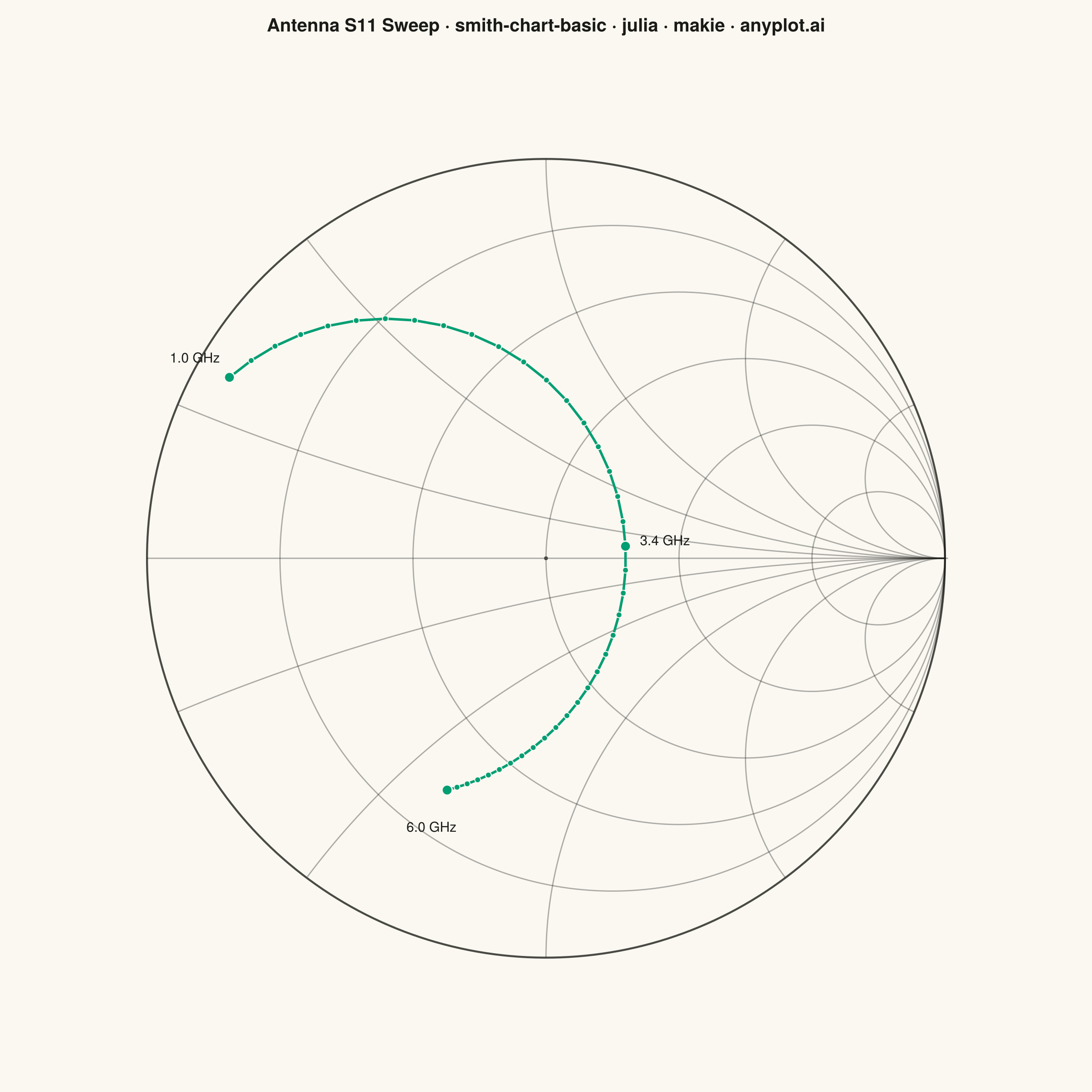
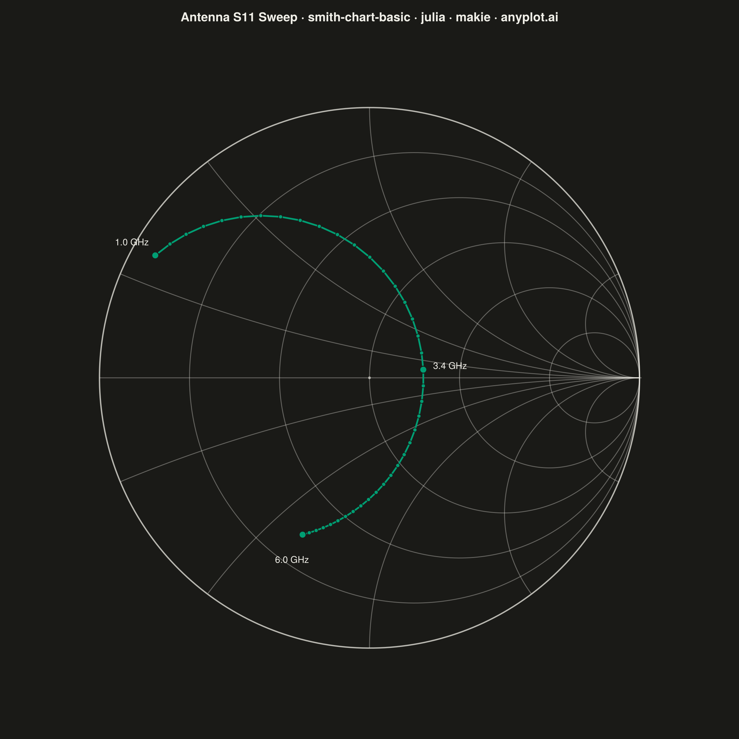
A Smith chart is a specialized circular diagram used in RF engineering to display complex impedance and reflection coefficients on a normalized polar grid. The chart features constant resistance circles (centered along the horizontal axis) and constant reactance arcs (curving from the right edge), enabling engineers to visualize impedance matching, transmission line behavior, and antenna characteristics. It reveals relationships between impedance, admittance, and reflection coefficient that would be difficult to interpret in Cartesian coordinates.
# anyplot.ai
# smith-chart-basic: Smith Chart for RF/Impedance
# Library: makie 0.21.9 | Julia 1.11.9
# Quality: 90/100 | Created: 2026-09-02

using CairoMakie
using Colors

# Theme tokens — Imprint palette, theme-adaptive chrome
const THEME    = get(ENV, "ANYPLOT_THEME", "light")
const PAGE_BG  = THEME == "light" ? colorant"#FAF8F1" : colorant"#1A1A17"
const INK      = THEME == "light" ? colorant"#1A1A17" : colorant"#F0EFE8"
const INK_SOFT = THEME == "light" ? colorant"#4A4A44" : colorant"#B8B7B0"
const BRAND    = colorant"#009E73"  # Imprint palette position 1 — always first series
const GRID     = RGBAf(INK.r, INK.g, INK.b, 0.35)

# Data — antenna feed impedance across a parallel-RLC resonance (S11 sweep, 1-6 GHz)
const z0          = 50.0       # reference impedance, ohms
const resistance  = 75.0       # radiation resistance, ohms
const inductance  = 2.0e-9     # feed inductance, H
const capacitance = 1.034e-12  # feed capacitance, F — tuned for resonance near 3.5 GHz

const n_points      = 40
const frequency_hz  = collect(range(1.0e9, 6.0e9, length = n_points))
const frequency_ghz = frequency_hz ./ 1.0e9
const omega         = 2π .* frequency_hz

const admittance = (1 / resistance) .+ (im .* omega .* capacitance) .+
                   (1 ./ (im .* omega .* inductance))
const impedance = 1 ./ admittance
const z_real    = real.(impedance)
const z_imag    = imag.(impedance)

const z_norm   = (z_real .+ im .* z_imag) ./ z0
const gamma    = (z_norm .- 1) ./ (z_norm .+ 1)
const gamma_re = real.(gamma)
const gamma_im = imag.(gamma)

# Smith chart grid geometry
const n_circle  = 300
const theta     = range(0.0, 2π, length = n_circle)
const r_values  = [0.2, 0.5, 1.0, 2.0, 5.0]  # constant-resistance circles
const x_values  = [0.2, 0.5, 1.0, 2.0, 5.0]  # constant-reactance arcs (±)
const n_arc     = 2000

# Title — fontsize scales down for titles longer than the 67-char baseline
title_str  = "Antenna S11 Sweep · smith-chart-basic · julia · makie · anyplot.ai"
n_title    = length(title_str)
title_size = round(Int, 20 * (n_title > 67 ? 67.0 / n_title : 1.0))

# Figure — square canvas (2400×2400 via px_per_unit=2): a Smith chart is a
# circular diagram with no preferred horizontal axis
fig = Figure(
    size            = (1200, 1200),
    fontsize        = 14,
    backgroundcolor = PAGE_BG,
)

ax = Axis(
    fig[1, 1];
    title              = title_str,
    titlesize          = title_size,
    titlecolor         = INK,
    backgroundcolor    = PAGE_BG,
    aspect             = DataAspect(),
    xgridvisible       = false,
    ygridvisible       = false,
    xticksvisible      = false,
    yticksvisible      = false,
    xticklabelsvisible = false,
    yticklabelsvisible = false,
    leftspinevisible   = false,
    rightspinevisible  = false,
    topspinevisible    = false,
    bottomspinevisible = false,
)

xlims!(ax, -1.3, 1.3)
ylims!(ax, -1.3, 1.3)

# Chart boundary — |Γ| = 1, total reflection
lines!(ax, cos.(theta), sin.(theta); color = INK_SOFT, linewidth = 2.2)

# Zero-reactance diameter — the matched condition Z = Z0 sits at the origin
lines!(ax, [-1.0, 1.0], [0.0, 0.0]; color = GRID, linewidth = 1.4)

# Constant-resistance circles r = 0.2, 0.5, 1, 2, 5 — always fully inside the unit disk
for r in r_values
    cx     = r / (1 + r)
    radius = 1 / (1 + r)
    lines!(ax, cx .+ radius .* cos.(theta), radius .* sin.(theta);
        color = GRID, linewidth = 1.4)
end

# Constant-reactance arcs x = ±0.2, ±0.5, ±1, ±2, ±5 — trimmed to the unit disk.
# Every such circle passes through Γ = 1; the disk-interior stretch is found by
# walking outward from that anchor point in both angular directions.
for x in vcat(x_values, -x_values)
    rc     = 1.0 / x
    radius = abs(rc)
    anchor = rc > 0 ? -π / 2 : π / 2
    psi    = range(-π, π, length = n_arc)
    phi    = anchor .+ psi
    px     = 1.0 .+ radius .* cos.(phi)
    py     = rc .+ radius .* sin.(phi)
    inside = (px .^ 2 .+ py .^ 2) .<= 1.0 + 1.0e-6

    mid = n_arc ÷ 2 + 1
    lo, hi = mid, mid
    while lo > 1 && inside[lo - 1]
        lo -= 1
    end
    while hi < n_arc && inside[hi + 1]
        hi += 1
    end

    lines!(ax, px[lo:hi], py[lo:hi]; color = GRID, linewidth = 1.4)
end

# Matched-condition point — Z = Z0, Γ = 0
scatter!(ax, [0.0], [0.0]; color = INK_SOFT, markersize = 6, strokewidth = 0)

# Impedance locus — antenna feed impedance trajectory across the frequency sweep
lines!(ax, gamma_re, gamma_im; color = BRAND, linewidth = 2.75)
scatter!(ax, gamma_re, gamma_im;
    color = BRAND, markersize = 9, strokewidth = 1.0, strokecolor = PAGE_BG)

# Frequency labels at key points along the locus
label_idx = [1, round(Int, n_points / 2), n_points]
for i in label_idx
    gx, gy       = gamma_re[i], gamma_im[i]
    r_i          = hypot(gx, gy)
    dir_x, dir_y = r_i > 1.0e-6 ? (gx / r_i, gy / r_i) : (1.0, 0.0)
    lx, ly       = gx + 0.10 * dir_x, gy + 0.10 * dir_y

    scatter!(ax, [gx], [gy];
        color = BRAND, markersize = 16, strokewidth = 1.5, strokecolor = PAGE_BG)
    text!(ax, lx, ly; text = "$(round(frequency_ghz[i], digits = 1)) GHz",
        color = INK, fontsize = 15, align = (:center, :center))
end

# Save
save("plot-$(THEME).png", fig; px_per_unit = 2)
Runnable source as JSON, for any HTTP client: https://api.anyplot.ai/specs/smith-chart-basic/makie/code. Any spec id and library id listed in llms-full.txt fit the same URL shape; every URL below is complete and callable.
{
  "spec_id": "smith-chart-basic",
  "language": "julia",
  "library": "makie",
  "page": "https://anyplot.ai/smith-chart-basic/julia/makie",
  "hub": "https://anyplot.ai/smith-chart-basic",
  "code_json": "https://api.anyplot.ai/specs/smith-chart-basic/makie/code",
  "spec_json": "https://api.anyplot.ai/specs/smith-chart-basic",
  "render_light_png": "https://storage.googleapis.com/anyplot-images/plots/smith-chart-basic/julia/makie/plot-light.png",
  "render_dark_png": "https://storage.googleapis.com/anyplot-images/plots/smith-chart-basic/julia/makie/plot-dark.png",
  "quality_score": 90.0,
  "license": "MIT",
  "guide": "https://anyplot.ai/llms.txt"
}
Part of Smith Chart for RF/Impedance on anyplot.ai.