The same plot in 14 other libraries — JavaScript: Chart.js, D3.js, Apache ECharts, Highcharts; Python: Altair, Bokeh, lets-plot, Matplotlib, Plotly, plotnine, Pygal, Seaborn; R: ggplot2; Julia: Makie.jl. Compare all 15 side by side: Smith Chart for RF/Impedance in Python, R, Julia and JavaScript.
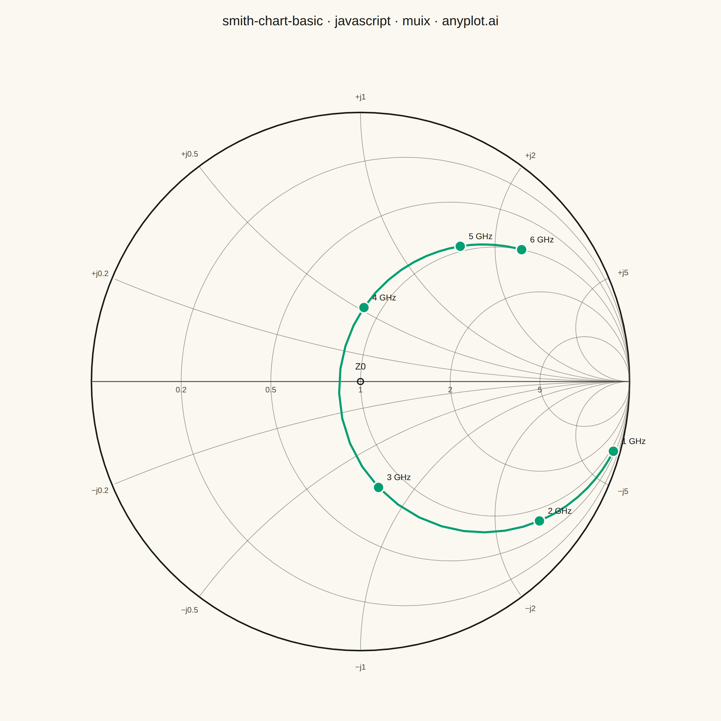
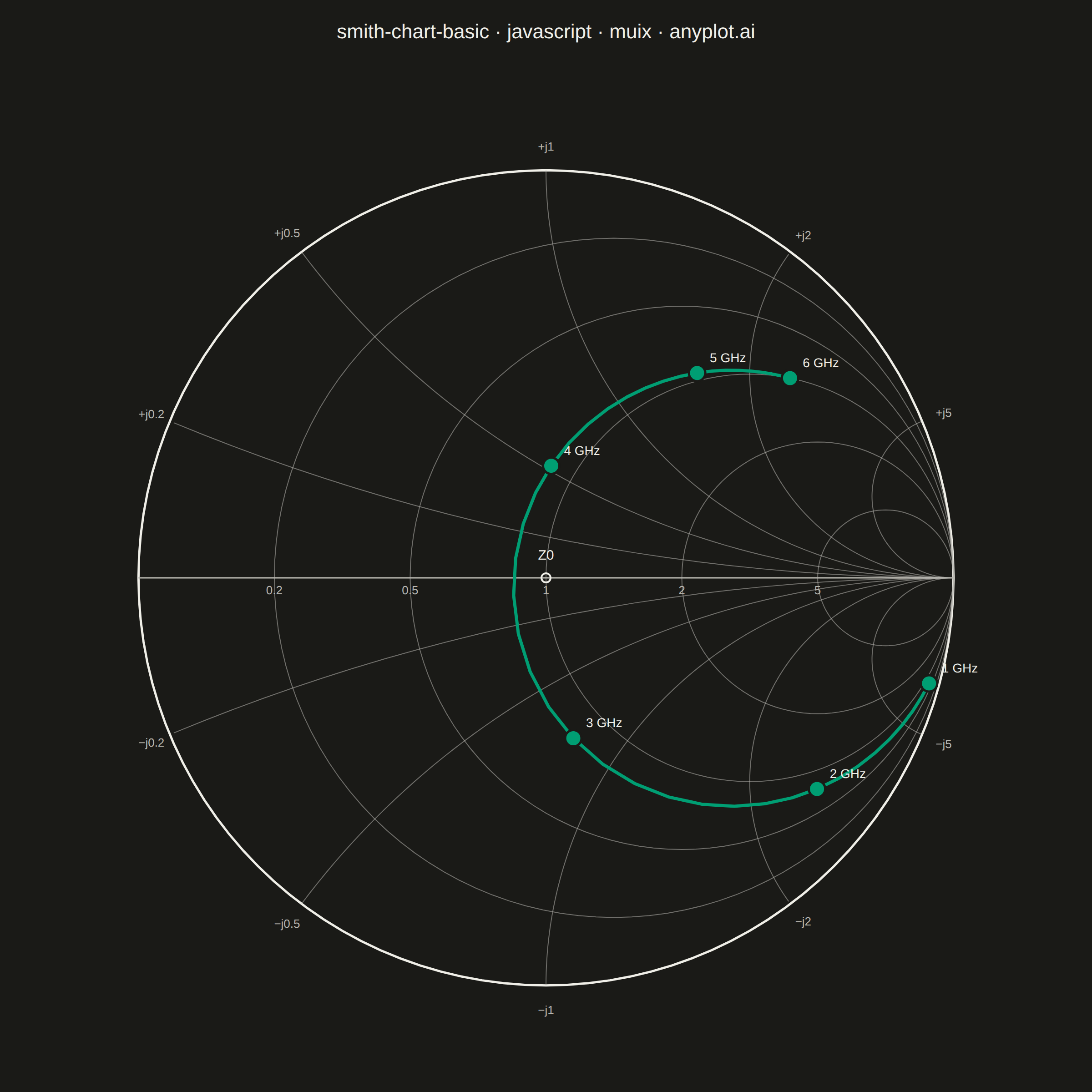
A Smith chart is a specialized circular diagram used in RF engineering to display complex impedance and reflection coefficients on a normalized polar grid. The chart features constant resistance circles (centered along the horizontal axis) and constant reactance arcs (curving from the right edge), enabling engineers to visualize impedance matching, transmission line behavior, and antenna characteristics. It reveals relationships between impedance, admittance, and reflection coefficient that would be difficult to interpret in Cartesian coordinates.
// anyplot.ai
// smith-chart-basic: Smith Chart for RF/Impedance
// Library: muix 7.29.1 | JavaScript 22.23.2
// Quality: 89/100 | Created: 2026-09-02
//# anyplot-orientation: square
// anyplot.ai
// smith-chart-basic: Smith Chart for RF/Impedance
// Library: MUI X Charts | React | Node 22
// License: @mui/x-charts — MIT (community). Pro/Premium are out of scope.
// Quality: pending | Created: 2026-09-02
import { ChartContainer } from "@mui/x-charts/ChartContainer";
import { ChartsText } from "@mui/x-charts/ChartsText";
import { useXScale, useYScale } from "@mui/x-charts/hooks";

const t = window.ANYPLOT_TOKENS;

// --- Antenna feed impedance sweep (in-memory, deterministic RLC model) ------
// A series R-L-C feed model: radiation resistance rises gently with
// frequency while the reactance swings through resonance — a textbook
// Smith-chart trajectory for a monopole antenna matched to Z0.
const Z0 = 50; // ohms — reference impedance
const INDUCTANCE = 5e-9; // henries — series feed inductance
const CAPACITANCE = 0.4e-12; // farads — series feed capacitance
const FREQ_START_GHZ = 1;
const FREQ_END_GHZ = 6;
const FREQ_STEP_GHZ = 0.125;

const frequenciesGHz = [];
for (let f = FREQ_START_GHZ; f <= FREQ_END_GHZ + 1e-9; f += FREQ_STEP_GHZ) {
  frequenciesGHz.push(Math.round(f * 1000) / 1000);
}

const gammaPoints = frequenciesGHz.map((fGHz) => {
  const omega = 2 * Math.PI * fGHz * 1e9;
  const resistance = 35 + 3 * (fGHz - FREQ_START_GHZ);
  const reactance = omega * INDUCTANCE - 1 / (omega * CAPACITANCE);
  const zReal = resistance / Z0;
  const zImag = reactance / Z0;
  // gamma = (z_norm - 1) / (z_norm + 1), complex division done by hand
  const denomReal = zReal + 1;
  const denomImag = zImag;
  const denomMagSq = denomReal * denomReal + denomImag * denomImag;
  const numReal = zReal - 1;
  const numImag = zImag;
  return {
    fGHz,
    re: (numReal * denomReal + numImag * denomImag) / denomMagSq,
    im: (numImag * denomReal - numReal * denomImag) / denomMagSq,
  };
});
const labeledFreqs = [1, 2, 3, 4, 5, 6];

// --- Smith-chart grid geometry (unit circle in the Γ-plane) -----------------
const RESISTANCE_VALUES = [0.2, 0.5, 1, 2, 5];
const REACTANCE_VALUES = [0.2, 0.5, 1, 2, 5];
const GAMMA_MAX = 1.15;
const CIRCLE_STEPS = 120;

const circlePoints = (cx, cy, r, steps = CIRCLE_STEPS) =>
  Array.from({ length: steps + 1 }, (_, i) => {
    const theta = (i / steps) * 2 * Math.PI;
    return [cx + r * Math.cos(theta), cy + r * Math.sin(theta)];
  });

// Every constant-reactance circle passes through the open-circuit point
// (1, 0); only the portion that curves back into the unit disk belongs on
// the chart. That portion's angular span depends on the circle's radius
// (tiny for large |x|, most of the circle for small |x|), so it is found by
// walking outward from (1, 0) until the circle re-crosses |Γ| = 1, rather
// than assumed to be a fixed half-circle.
const reactanceArcPoints = (xVal, steps = 400) => {
  const cx = 1;
  const cy = 1 / xVal;
  const r = Math.abs(1 / xVal);
  const theta0 = Math.atan2(-cy, 0);
  const pointAt = (theta) => [cx + r * Math.cos(theta), cy + r * Math.sin(theta)];
  const norm2 = ([x, y]) => x * x + y * y;
  const dTheta = (2 * Math.PI) / steps;
  const direction = norm2(pointAt(theta0 + dTheta)) < norm2(pointAt(theta0 - dTheta)) ? 1 : -1;
  const points = [pointAt(theta0)];
  for (let i = 1; i <= steps; i++) {
    const p = pointAt(theta0 + direction * dTheta * i);
    if (norm2(p) > 1.0005) break;
    points.push(p);
  }
  return points;
};

const pathFromPoints = (points, toPx) =>
  points
    .map(([x, y], i) => {
      const p = toPx(x, y);
      return `${i === 0 ? "M" : "L"} ${p.x} ${p.y}`;
    })
    .join(" ");

// --- Overlay: resistance circles, reactance arcs, matched-center marker -----
// Community `@mui/x-charts/hooks` (useXScale/useYScale) map Γ-plane
// coordinates to pixels so the grid stays aligned with the locus at any size.
function SmithGrid() {
  const xScale = useXScale();
  const yScale = useYScale();
  const toPx = (re, im) => ({ x: xScale(re), y: yScale(im) });

  return (
    <g>
      <path d={pathFromPoints(circlePoints(0, 0, 1), toPx)} fill="none" stroke={t.ink} strokeWidth={2.5} />
      <line
        x1={toPx(-1, 0).x}
        y1={toPx(-1, 0).y}
        x2={toPx(1, 0).x}
        y2={toPx(1, 0).y}
        stroke={t.inkSoft}
        strokeWidth={1.5}
      />
      {RESISTANCE_VALUES.map((r) => (
        <path
          key={`r-${r}`}
          d={pathFromPoints(circlePoints(r / (1 + r), 0, 1 / (1 + r)), toPx)}
          fill="none"
          stroke={t.inkSoft}
          strokeWidth={1}
          opacity={0.55}
        />
      ))}
      {REACTANCE_VALUES.flatMap((x) => [x, -x]).map((x) => (
        <path
          key={`x-${x}`}
          d={pathFromPoints(reactanceArcPoints(x), toPx)}
          fill="none"
          stroke={t.inkSoft}
          strokeWidth={1}
          opacity={0.55}
        />
      ))}
      {RESISTANCE_VALUES.map((r) => {
        const p = toPx((r - 1) / (1 + r), 0);
        // r=1 sits exactly at the chart center, right next to the Z0 marker —
        // give it extra clearance so the two labels don't cluster together.
        const labelOffset = r === 1 ? 26 : 18;
        return (
          <ChartsText
            key={`rl-${r}`}
            x={p.x}
            y={p.y + labelOffset}
            text={String(r)}
            style={{ fontSize: 13, fill: t.inkSoft, textAnchor: "middle" }}
          />
        );
      })}
      {REACTANCE_VALUES.flatMap((x) => [x, -x]).map((x) => {
        // Label at the arc's outer end (where it re-crosses the boundary),
        // nudged further out along the same radial direction from origin.
        const arcPoints = reactanceArcPoints(x);
        const [ax, ay] = arcPoints[arcPoints.length - 1];
        const p = toPx(ax * 1.06, ay * 1.06);
        return (
          <ChartsText
            key={`xl-${x}`}
            x={p.x}
            y={p.y}
            text={`${x > 0 ? "+j" : "−j"}${Math.abs(x)}`}
            style={{ fontSize: 13, fill: t.inkSoft, textAnchor: "middle", dominantBaseline: "central" }}
          />
        );
      })}
      <circle cx={toPx(0, 0).x} cy={toPx(0, 0).y} r={5} fill="none" stroke={t.ink} strokeWidth={2} />
      <ChartsText
        x={toPx(0, 0).x}
        y={toPx(0, 0).y - 26}
        text="Z0"
        style={{ fontSize: 15, fill: t.ink, textAnchor: "middle", fontWeight: 500 }}
      />
    </g>
  );
}

// --- Overlay: the swept impedance locus with frequency waypoints ------------
function ImpedanceLocus() {
  const xScale = useXScale();
  const yScale = useYScale();
  const toPx = (re, im) => ({ x: xScale(re), y: yScale(im) });
  const brand = t.palette[0];

  return (
    <g>
      <path
        d={pathFromPoints(
          gammaPoints.map((p) => [p.re, p.im]),
          toPx,
        )}
        fill="none"
        stroke={brand}
        strokeWidth={3.5}
        strokeLinecap="round"
        strokeLinejoin="round"
      />
      {gammaPoints
        .filter((p) => labeledFreqs.includes(p.fGHz))
        .map((p) => {
          const px = toPx(p.re, p.im);
          // Nudge the label outward along the radial direction from the chart
          // center (same technique as the reactance-arc labels above) rather
          // than a fixed pixel offset — points near |Γ|=1 (e.g. 1 GHz at
          // |Γ|≈0.975) would otherwise sit on top of the boundary circle and
          // converging grid arcs.
          const origin = toPx(0, 0);
          const dx = px.x - origin.x;
          const dy = px.y - origin.y;
          const dist = Math.hypot(dx, dy) || 1;
          const ux = dx / dist;
          const uy = dy / dist;
          const LABEL_OFFSET_PX = 26;
          const lx = px.x + ux * LABEL_OFFSET_PX;
          const ly = px.y + uy * LABEL_OFFSET_PX;
          return (
            <g key={p.fGHz}>
              <circle cx={px.x} cy={px.y} r={9} fill={brand} stroke={t.pageBg} strokeWidth={2.5} />
              <ChartsText
                x={lx}
                y={ly}
                text={`${p.fGHz} GHz`}
                style={{
                  fontSize: 14,
                  fill: t.ink,
                  fontWeight: 500,
                  textAnchor: ux >= 0.15 ? "start" : ux <= -0.15 ? "end" : "middle",
                  dominantBaseline: uy >= 0.15 ? "hanging" : uy <= -0.15 ? "auto" : "central",
                }}
              />
            </g>
          );
        })}
    </g>
  );
}

const TITLE = "smith-chart-basic · javascript · muix · anyplot.ai";
const TITLE_HEIGHT = 70;

// Left/right margin is derived so the drawing area is a perfect square —
// required for the Γ-plane circles to render as true circles, not ellipses.
const BASE_MARGIN = 50;
const chartHeight = window.ANYPLOT_SIZE.height - TITLE_HEIGHT;
const squareSide = chartHeight - 2 * BASE_MARGIN;
const sideMargin = (window.ANYPLOT_SIZE.width - squareSide) / 2;
const MARGIN = { top: BASE_MARGIN, bottom: BASE_MARGIN, left: sideMargin, right: sideMargin };

// --- Chart (default-exported component — the harness mounts it) -------------
export default function Chart() {
  return (
    <div
      style={{
        width: window.ANYPLOT_SIZE.width,
        height: window.ANYPLOT_SIZE.height,
        display: "flex",
        flexDirection: "column",
      }}
    >
      <div
        style={{
          height: TITLE_HEIGHT,
          display: "flex",
          alignItems: "center",
          justifyContent: "center",
          fontSize: 22,
          fontWeight: 500,
          color: t.ink,
        }}
      >
        {TITLE}
      </div>
      <ChartContainer
        width={window.ANYPLOT_SIZE.width}
        height={chartHeight}
        margin={MARGIN}
        series={[]}
        skipAnimation
        disableAxisListener
        xAxis={[{ scaleType: "linear", min: -GAMMA_MAX, max: GAMMA_MAX }]}
        yAxis={[{ scaleType: "linear", min: -GAMMA_MAX, max: GAMMA_MAX }]}
      >
        <SmithGrid />
        <ImpedanceLocus />
      </ChartContainer>
    </div>
  );
}
Runnable source as JSON, for any HTTP client: https://api.anyplot.ai/specs/smith-chart-basic/muix/code. Any spec id and library id listed in llms-full.txt fit the same URL shape; every URL below is complete and callable.
{
  "spec_id": "smith-chart-basic",
  "language": "javascript",
  "library": "muix",
  "page": "https://anyplot.ai/smith-chart-basic/javascript/muix",
  "hub": "https://anyplot.ai/smith-chart-basic",
  "code_json": "https://api.anyplot.ai/specs/smith-chart-basic/muix/code",
  "spec_json": "https://api.anyplot.ai/specs/smith-chart-basic",
  "render_light_png": "https://storage.googleapis.com/anyplot-images/plots/smith-chart-basic/javascript/muix/plot-light.png",
  "render_dark_png": "https://storage.googleapis.com/anyplot-images/plots/smith-chart-basic/javascript/muix/plot-dark.png",
  "interactive_light_html": "https://storage.googleapis.com/anyplot-images/plots/smith-chart-basic/javascript/muix/plot-light.html",
  "interactive_dark_html": "https://storage.googleapis.com/anyplot-images/plots/smith-chart-basic/javascript/muix/plot-dark.html",
  "quality_score": 89.0,
  "license": "MIT",
  "guide": "https://anyplot.ai/llms.txt"
}
Part of Smith Chart for RF/Impedance on anyplot.ai.