Smith Chart for RF/Impedance — Pygal

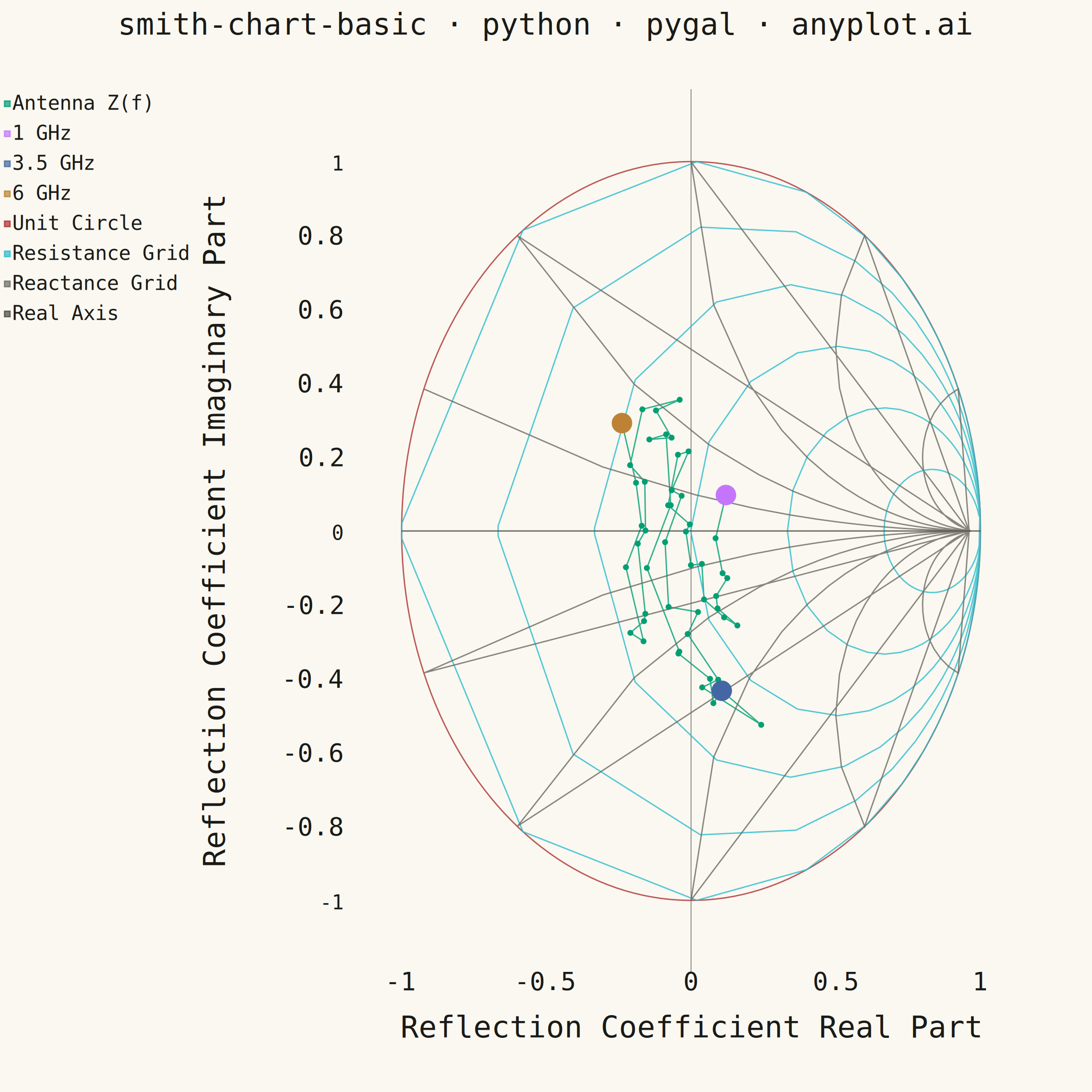
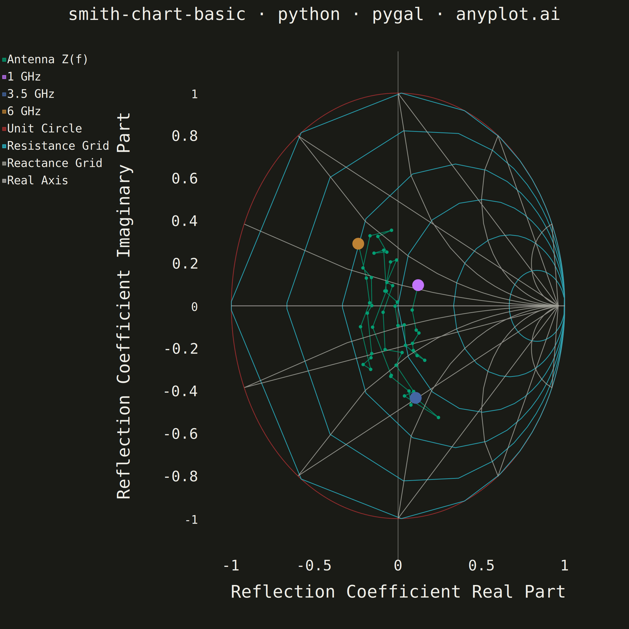
A Smith chart is a specialized circular diagram used in RF engineering to display complex impedance and reflection coefficients on a normalized polar grid. The chart features constant resistance circles (centered along the horizontal axis) and constant reactance arcs (curving from the right edge), enabling engineers to visualize impedance matching, transmission line behavior, and antenna characteristics. It reveals relationships between impedance, admittance, and reflection coefficient that would be difficult to interpret in Cartesian coordinates.

Smith Chart for RF/Impedance rendered with Pygal

Python source (Pygal)

""" anyplot.ai
smith-chart-basic: Smith Chart for RF/Impedance
Library: pygal 3.1.0 | Python 3.13.13
Quality: 83/100 | Updated: 2026-05-20
"""

import os

import numpy as np
import pygal
from pygal.style import Style


# Theme tokens
THEME = os.getenv("ANYPLOT_THEME", "light")
PAGE_BG = "#FAF8F1" if THEME == "light" else "#1A1A17"
INK = "#1A1A17" if THEME == "light" else "#F0EFE8"
INK_SOFT = "#4A4A44" if THEME == "light" else "#B8B7B0"
INK_MUTED = "#6B6A63" if THEME == "light" else "#A8A79F"

# Canonical Okabe-Ito order: data series take palette positions 1-4 (added first),
# structural chart elements use positions 5-8 (added after data).
CHART_COLORS = (
    "#009E73",  # pos 1: "Antenna Z(f)" ← brand green — first data series
    "#C475FD",  # pos 2: "1 GHz" (Okabe-Ito vermillion)
    "#4467A3",  # pos 3: "3.5 GHz" (Okabe-Ito blue)
    "#BD8233",  # pos 4: "6 GHz" (Okabe-Ito pink/purple)
    "#AE3030",  # pos 5: unit circle boundary (Okabe-Ito amber)
    "#2ABCCD",  # pos 6: resistance circles (Okabe-Ito sky blue)
    INK_MUTED,  # pos 7: reactance arcs (theme-adaptive muted)
    INK_SOFT,  # pos 8: real axis (theme-adaptive subtle)
)

Z0 = 50  # reference impedance (ohms)
R_CIRCLES = [0, 0.2, 0.5, 1, 2, 5]
X_ARCS = [0.2, 0.5, 1, 2, 5]

# Style
custom_style = Style(
    background=PAGE_BG,
    plot_background=PAGE_BG,
    foreground=INK,
    foreground_strong=INK,
    foreground_subtle=INK_MUTED,
    colors=CHART_COLORS,
    title_font_size=66,
    label_font_size=56,
    major_label_font_size=44,
    legend_font_size=44,
    value_font_size=36,
    stroke_width=3,
)

# Chart — square format; truncate_label=-1 prevents pygal from clipping tick text
chart = pygal.XY(
    width=2400,
    height=2400,
    style=custom_style,
    title="smith-chart-basic · python · pygal · anyplot.ai",
    show_legend=True,
    legend_at_bottom=False,
    show_x_guides=False,
    show_y_guides=False,
    x_title="Reflection Coefficient Real Part",
    y_title="Reflection Coefficient Imaginary Part",
    dots_size=8,
    range=(-1.15, 1.15),
    xrange=(-1.15, 1.15),
    margin=120,
    truncate_label=-1,
)

# Explicit tick marks at clean round values to prevent floating-point label truncation
chart.x_labels = [-1.0, -0.5, 0.0, 0.5, 1.0]

# Data — antenna impedance sweep 1–6 GHz
# Added FIRST so data series take palette positions 1-4 (brand green at pos 1)
np.random.seed(42)
n = 50
freqs = np.linspace(1e9, 6e9, n)

r_base = 25 + 50 * np.exp(-freqs / 3e9)
x_base = 30 * np.sin(2 * np.pi * freqs / 2e9) + 20 * np.cos(freqs / 1e9)
z_r = r_base + np.random.randn(n) * 3
z_i = x_base + np.random.randn(n) * 5

z_c = z_r + 1j * z_i
z_norm = z_c / Z0
gamma = (z_norm - 1) / (z_norm + 1)

# Impedance locus: pos 1 = #009E73 brand green
locus = [(float(g.real), float(g.imag)) for g in gamma]
chart.add("Antenna Z(f)", locus, show_dots=True, stroke_width=5, dots_size=6)

# Frequency markers (stroke=False = dots only, no connecting line): pos 2-4
chart.add("1 GHz", [(float(gamma[0].real), float(gamma[0].imag))], show_dots=True, dots_size=22, stroke=False)
chart.add(
    "3.5 GHz", [(float(gamma[n // 2].real), float(gamma[n // 2].imag))], show_dots=True, dots_size=22, stroke=False
)
chart.add("6 GHz", [(float(gamma[-1].real), float(gamma[-1].imag))], show_dots=True, dots_size=22, stroke=False)

# Structural series — added AFTER data to take palette positions 5-8.
# Named labels eliminate the unlabeled colored squares that caused legend confusion.
# Unit circle boundary (|Γ| = 1): pos 5 = #AE3030 amber
theta = np.linspace(0, 2 * np.pi, 200)
unit_circle = [(float(np.cos(t)), float(np.sin(t))) for t in theta]
chart.add("Unit Circle", unit_circle, show_dots=False, stroke_width=5)

# Constant resistance circles: pos 6 = #2ABCCD sky blue
r_grid = []
for r in R_CIRCLES:
    x_vals = np.concatenate([np.linspace(-50, -0.01, 100), np.linspace(0.01, 50, 100)])
    for x in x_vals:
        z_n = complex(r, x)
        g = (z_n - 1) / (z_n + 1)
        if abs(g) <= 1.001:
            r_grid.append((float(g.real), float(g.imag)))
    r_grid.append((None, None))
chart.add("Resistance Grid", r_grid, show_dots=False, stroke_width=1.5)

# Constant reactance arcs: pos 7 = INK_MUTED gray
x_grid = []
for x in X_ARCS:
    for r in np.linspace(0.001, 50, 100):
        z_n = complex(r, x)
        g = (z_n - 1) / (z_n + 1)
        if abs(g) <= 1.001:
            x_grid.append((float(g.real), float(g.imag)))
    x_grid.append((None, None))
    for r in np.linspace(0.001, 50, 100):
        z_n = complex(r, -x)
        g = (z_n - 1) / (z_n + 1)
        if abs(g) <= 1.001:
            x_grid.append((float(g.real), float(g.imag)))
    x_grid.append((None, None))
chart.add("Reactance Grid", x_grid, show_dots=False, stroke_width=1.5)

# Real axis: pos 8 = INK_SOFT gray
chart.add("Real Axis", [(-1.0, 0.0), (1.0, 0.0)], show_dots=False, stroke_width=2)

# Save
chart.render_to_file(f"plot-{THEME}.html")
chart.render_to_png(f"plot-{THEME}.png")

Part of Smith Chart for RF/Impedance on anyplot.ai.

Smith Chart for RF/Impedance — Pygal

Python source (Pygal)

Other implementations