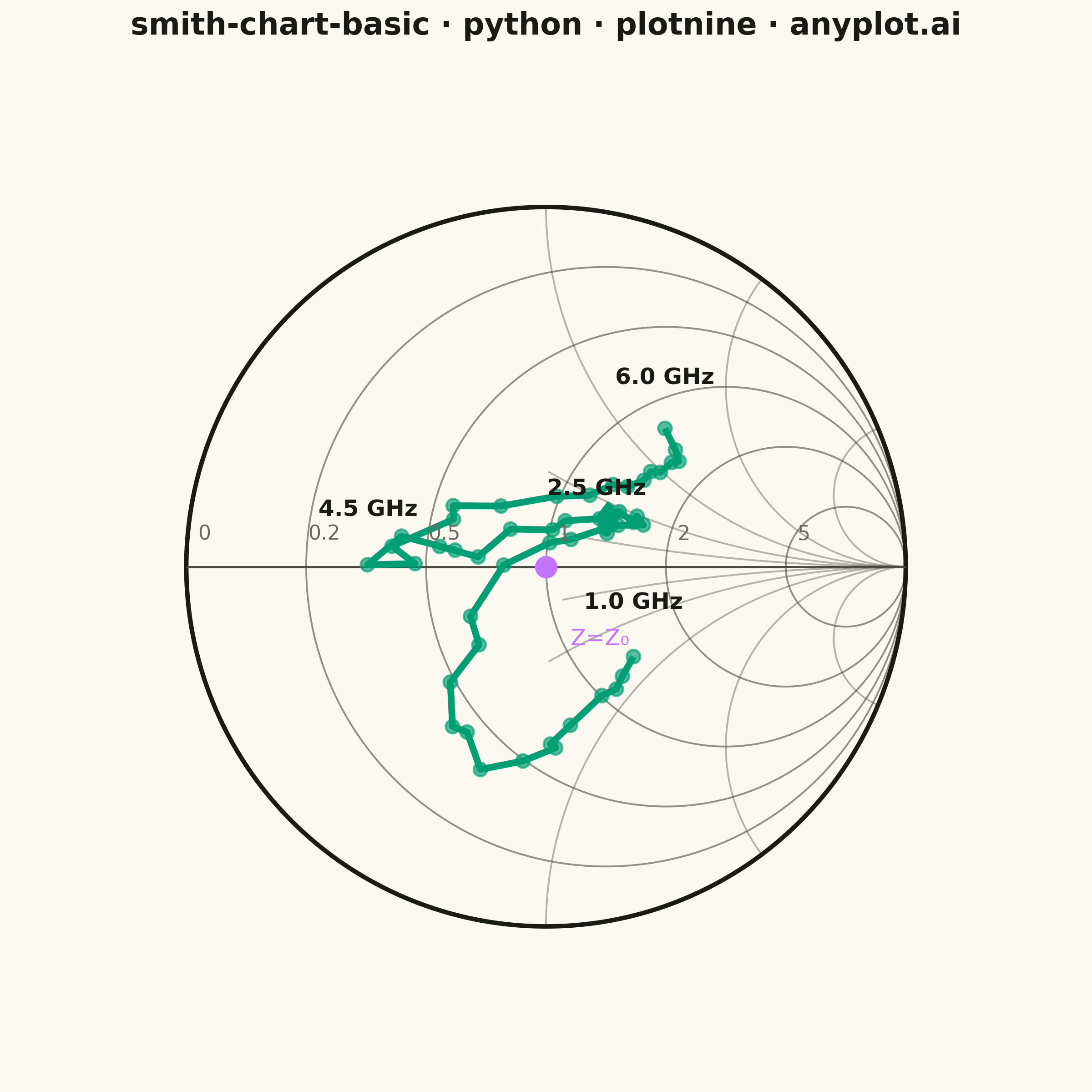
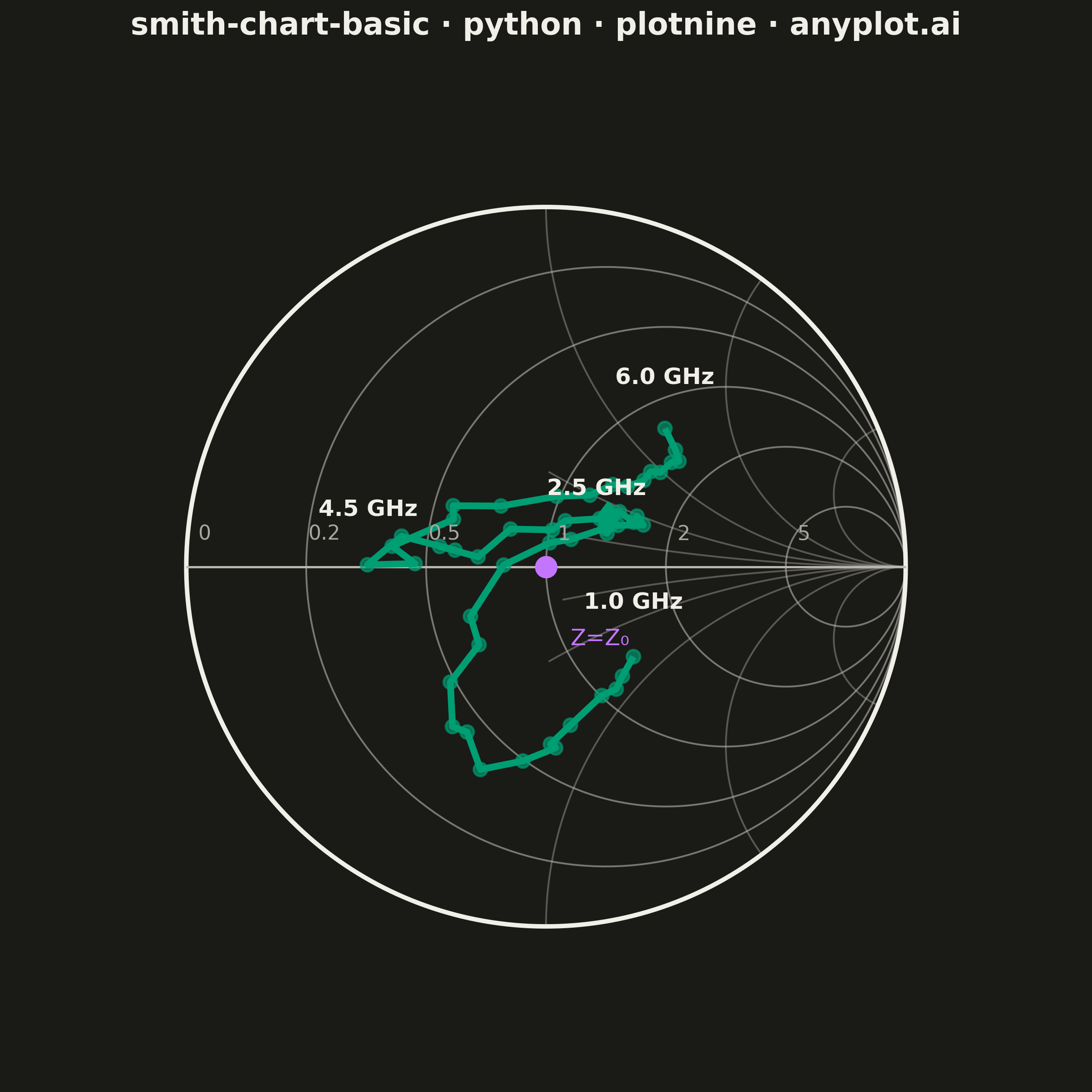
A Smith chart is a specialized circular diagram used in RF engineering to display complex impedance and reflection coefficients on a normalized polar grid. The chart features constant resistance circles (centered along the horizontal axis) and constant reactance arcs (curving from the right edge), enabling engineers to visualize impedance matching, transmission line behavior, and antenna characteristics. It reveals relationships between impedance, admittance, and reflection coefficient that would be difficult to interpret in Cartesian coordinates.
""" anyplot.ai
smith-chart-basic: Smith Chart for RF/Impedance
Library: plotnine 0.15.4 | Python 3.13.13
Quality: 89/100 | Updated: 2026-05-20
"""

import os

import numpy as np
import pandas as pd
from plotnine import (
    aes,
    annotate,
    arrow,
    coord_fixed,
    element_blank,
    element_rect,
    element_text,
    geom_path,
    geom_point,
    geom_segment,
    geom_text,
    ggplot,
    labs,
    scale_x_continuous,
    scale_y_continuous,
    theme,
)


# Theme tokens
THEME = os.getenv("ANYPLOT_THEME", "light")
PAGE_BG = "#FAF8F1" if THEME == "light" else "#1A1A17"
INK = "#1A1A17" if THEME == "light" else "#F0EFE8"
INK_SOFT = "#4A4A44" if THEME == "light" else "#B8B7B0"
INK_MUTED = "#6B6A63" if THEME == "light" else "#A8A79F"

IMPRINT = ["#009E73", "#C475FD", "#4467A3", "#BD8233", "#AE3030", "#2ABCCD", "#954477"]

# Data — Smith chart grid
Z0 = 50
r_values = [0, 0.2, 0.5, 1, 2, 5]
theta = np.linspace(0, 2 * np.pi, 200)

r_circle_data = []
for r in r_values:
    cx = r / (r + 1)
    radius = 1 / (r + 1)
    x = cx + radius * np.cos(theta)
    y = radius * np.sin(theta)
    mask = x**2 + y**2 <= 1.001
    r_circle_data.append(pd.DataFrame({"x": x[mask], "y": y[mask], "grp": f"r_{r}"}))
r_circles_df = pd.concat(r_circle_data, ignore_index=True)

x_values = [0.2, 0.5, 1, 2, 5]
reactance_data = []
for xv in x_values:
    radius_x = 1 / abs(xv)
    t = np.linspace(0, 2 * np.pi, 500)
    arc_x = 1 + radius_x * np.cos(t)
    for sign, tag in [(1, "p"), (-1, "n")]:
        arc_y = (sign / xv) + radius_x * np.sin(t)
        mask = (arc_x**2 + arc_y**2 <= 1.001) & (arc_x >= -0.01)
        if np.any(mask):
            reactance_data.append(pd.DataFrame({"x": arc_x[mask], "y": arc_y[mask], "grp": f"x_{tag}_{xv}"}))
reactance_df = pd.concat(reactance_data, ignore_index=True)

boundary_theta = np.linspace(0, 2 * np.pi, 300)
boundary_df = pd.DataFrame({"x": np.cos(boundary_theta), "y": np.sin(boundary_theta)})
axis_df = pd.DataFrame({"x": [-1.0, 1.0], "y": [0.0, 0.0]})

# Patch antenna S11 measurement from 1–6 GHz
np.random.seed(42)
n_points = 50
freq_ghz = np.linspace(1, 6, n_points)
z_real = 50 + 30 * np.sin(2 * np.pi * freq_ghz / 2.5) + np.random.randn(n_points) * 3
z_imag = 20 * np.cos(2 * np.pi * freq_ghz / 3) + 15 * (freq_ghz - 3) + np.random.randn(n_points) * 2

z_norm = (z_real + 1j * z_imag) / Z0
gamma = (z_norm - 1) / (z_norm + 1)
impedance_df = pd.DataFrame({"x": np.real(gamma), "y": np.imag(gamma), "freq": freq_ghz})

# Frequency labels at 4 key points with per-label nudges to prevent crowding
label_freqs = [1.0, 2.5, 4.5, 6.0]
label_idx = [int(np.argmin(np.abs(freq_ghz - f))) for f in label_freqs]
labels_df = impedance_df.iloc[label_idx].copy()
labels_df["label"] = [f"{f:.1f} GHz" for f in label_freqs]

# Per-label offsets: nudge 2.5/4.5 GHz apart horizontally; push 1.0 GHz up to clear Z=Z0 text
x_nudges = np.array([0.00, 0.13, -0.13, 0.00])
y_nudges = np.array([0.15, 0.15, 0.15, 0.14])
labels_df["x_label"] = labels_df["x"].values + x_nudges
labels_df["y_label"] = labels_df["y"].values + y_nudges

# Resistance circle labels just above the real axis at each circle's leftmost point
r_label_rows = [{"x": (r - 1) / (r + 1) + 0.05, "y": 0.09, "label": str(r)} for r in r_values]
r_labels_df = pd.DataFrame(r_label_rows)

# Mid-locus directional arrow (index 23→25) to indicate increasing frequency direction
arr_df = pd.DataFrame(
    {
        "x": [float(impedance_df.iloc[23]["x"])],
        "xend": [float(impedance_df.iloc[25]["x"])],
        "y": [float(impedance_df.iloc[23]["y"])],
        "yend": [float(impedance_df.iloc[25]["y"])],
    }
)

# Plot
plot = (
    ggplot()
    + geom_path(aes(x="x", y="y", group="grp"), data=r_circles_df, color=INK_SOFT, size=0.4, alpha=0.6)
    + geom_path(aes(x="x", y="y", group="grp"), data=reactance_df, color=INK_SOFT, size=0.4, alpha=0.4)
    + geom_path(aes(x="x", y="y"), data=boundary_df, color=INK, size=1.0)
    + geom_path(aes(x="x", y="y"), data=axis_df, color=INK_SOFT, size=0.5)
    + geom_path(aes(x="x", y="y"), data=impedance_df, color=IMPRINT[0], size=1.5)
    + geom_point(aes(x="x", y="y"), data=impedance_df, color=IMPRINT[0], size=2.5, alpha=0.65)
    + geom_segment(
        aes(x="x", xend="xend", y="y", yend="yend"), data=arr_df, color=IMPRINT[0], size=2.0, arrow=arrow(length=0.10)
    )
    + geom_text(aes(x="x_label", y="y_label", label="label"), data=labels_df, color=INK, size=9, fontweight="bold")
    + geom_text(aes(x="x", y="y", label="label"), data=r_labels_df, color=INK_MUTED, size=8)
    + annotate("point", x=0, y=0, color=IMPRINT[1], size=4)
    + annotate("text", x=0.15, y=-0.20, label="Z=Z₀", color=IMPRINT[1], size=9)
    + coord_fixed(ratio=1, xlim=(-1.3, 1.3), ylim=(-1.3, 1.3))
    + scale_x_continuous(breaks=[])
    + scale_y_continuous(breaks=[])
    + labs(title="smith-chart-basic · python · plotnine · anyplot.ai", x="", y="")
    + theme(
        figure_size=(6, 6),
        plot_title=element_text(size=12, ha="center", color=INK, fontweight="bold"),
        plot_background=element_rect(fill=PAGE_BG, color=PAGE_BG),
        panel_background=element_rect(fill=PAGE_BG),
        panel_grid_major=element_blank(),
        panel_grid_minor=element_blank(),
        axis_text=element_blank(),
        axis_ticks=element_blank(),
        axis_title=element_text(color=INK),
    )
)

plot.save(f"plot-{THEME}.png", dpi=400, width=6, height=6, units="in")
Runnable source as JSON, for any HTTP client: https://api.anyplot.ai/specs/smith-chart-basic/plotnine/code. Any spec id and library id listed in llms-full.txt fit the same URL shape; every URL below is complete and callable.
{
  "spec_id": "smith-chart-basic",
  "language": "python",
  "library": "plotnine",
  "page": "https://anyplot.ai/smith-chart-basic/python/plotnine",
  "hub": "https://anyplot.ai/smith-chart-basic",
  "code_json": "https://api.anyplot.ai/specs/smith-chart-basic/plotnine/code",
  "spec_json": "https://api.anyplot.ai/specs/smith-chart-basic",
  "render_light_png": "https://storage.googleapis.com/anyplot-images/plots/smith-chart-basic/python/plotnine/plot-light.png",
  "render_dark_png": "https://storage.googleapis.com/anyplot-images/plots/smith-chart-basic/python/plotnine/plot-dark.png",
  "quality_score": 89.0,
  "license": "MIT",
  "guide": "https://anyplot.ai/llms.txt"
}
Part of Smith Chart for RF/Impedance on anyplot.ai.