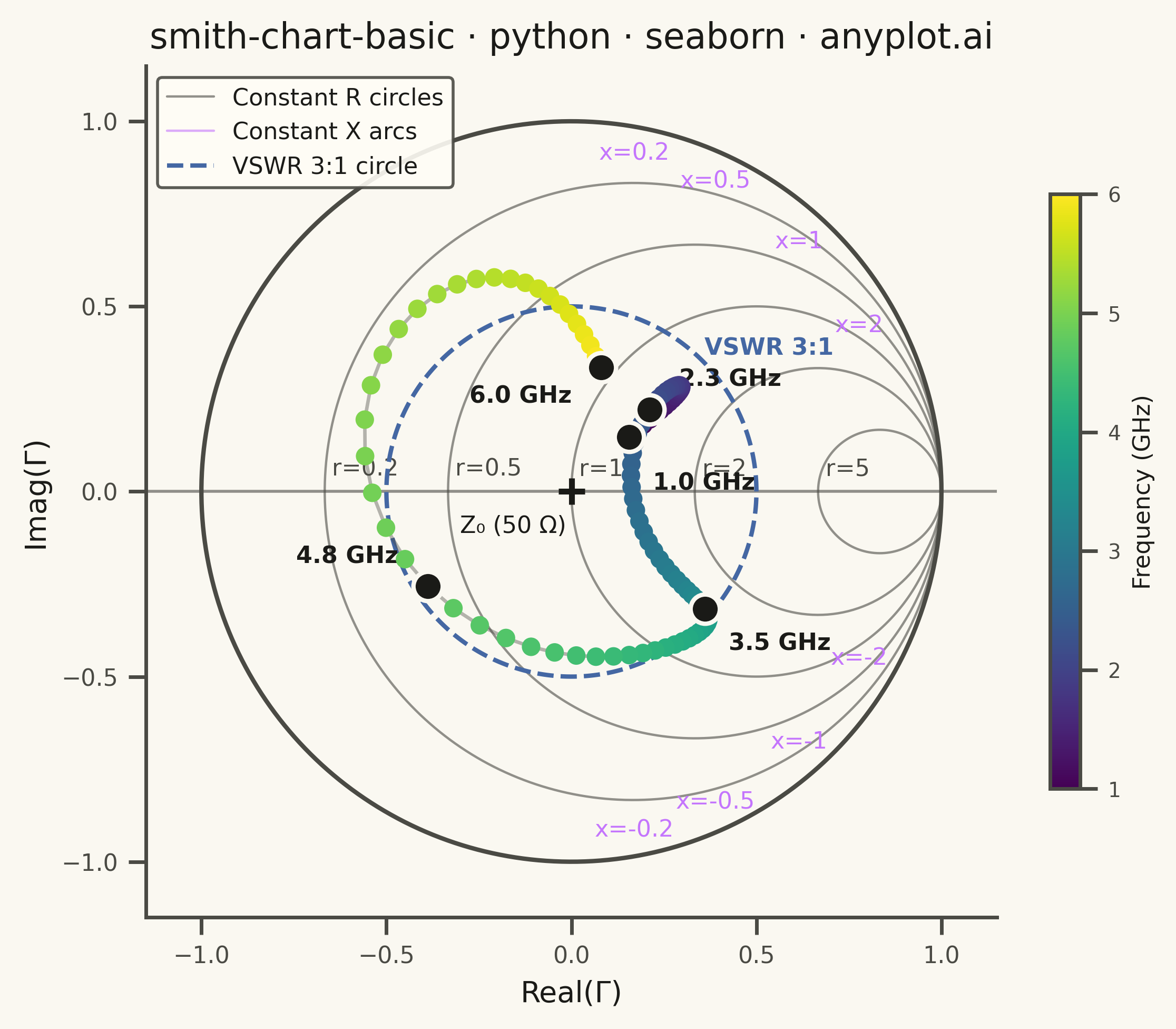
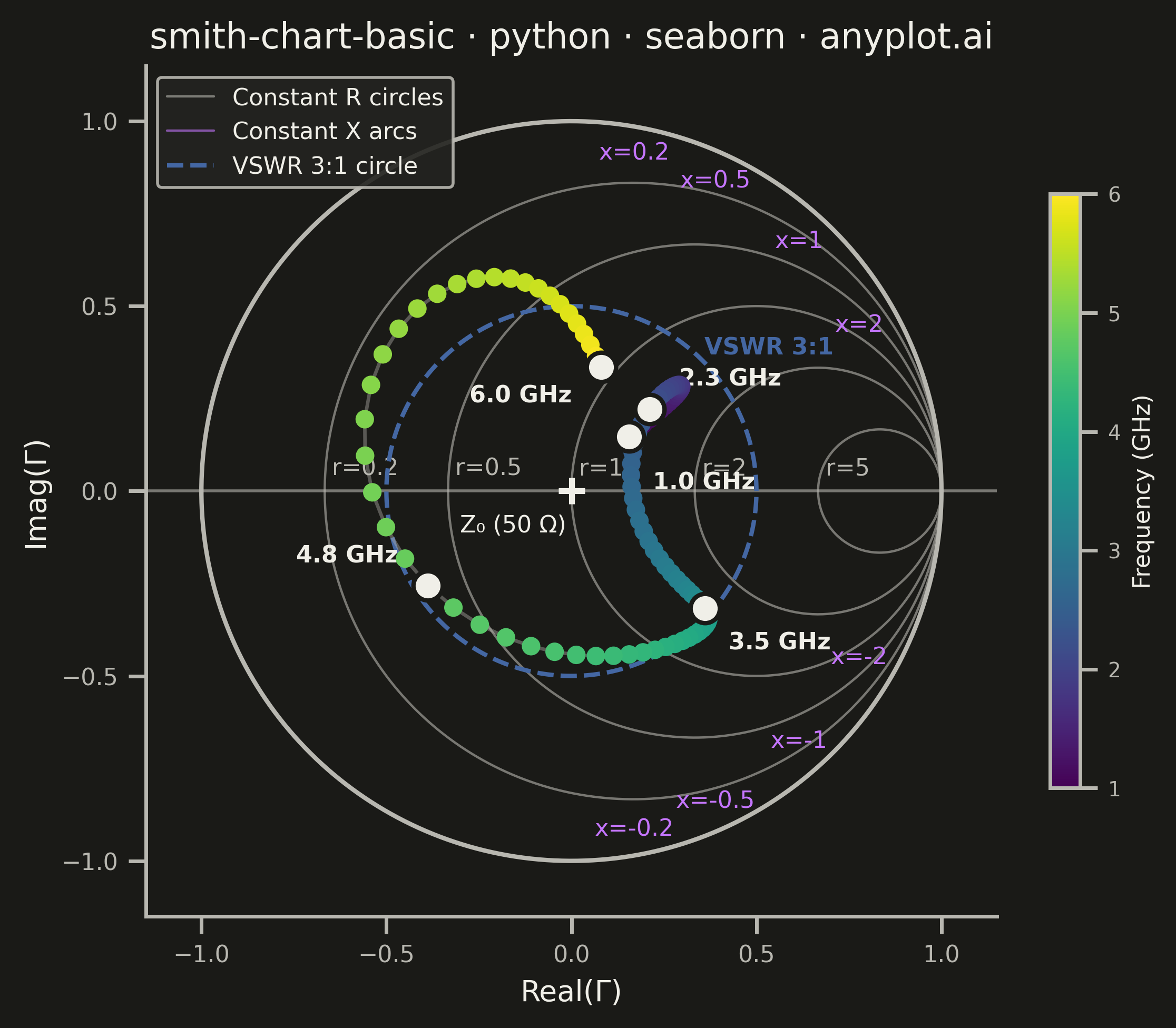
A Smith chart is a specialized circular diagram used in RF engineering to display complex impedance and reflection coefficients on a normalized polar grid. The chart features constant resistance circles (centered along the horizontal axis) and constant reactance arcs (curving from the right edge), enabling engineers to visualize impedance matching, transmission line behavior, and antenna characteristics. It reveals relationships between impedance, admittance, and reflection coefficient that would be difficult to interpret in Cartesian coordinates.
""" anyplot.ai
smith-chart-basic: Smith Chart for RF/Impedance
Library: seaborn 0.13.2 | Python 3.13.13
Quality: 86/100 | Updated: 2026-05-20
"""

import os

import matplotlib.pyplot as plt
import numpy as np
import pandas as pd
import seaborn as sns


# Theme tokens
THEME = os.getenv("ANYPLOT_THEME", "light")
PAGE_BG = "#FAF8F1" if THEME == "light" else "#1A1A17"
ELEVATED_BG = "#FFFDF6" if THEME == "light" else "#242420"
INK = "#1A1A17" if THEME == "light" else "#F0EFE8"
INK_SOFT = "#4A4A44" if THEME == "light" else "#B8B7B0"

# Okabe-Ito data colors (categorical series)
REACT_COLOR = "#C475FD"  # Reactance arcs — second series
VSWR_COLOR = "#4467A3"  # VSWR reference circle — third series

# Apply seaborn theme for chrome elements
sns.set_theme(
    style="ticks",
    rc={
        "figure.facecolor": PAGE_BG,
        "axes.facecolor": PAGE_BG,
        "axes.edgecolor": INK_SOFT,
        "axes.labelcolor": INK,
        "text.color": INK,
        "xtick.color": INK_SOFT,
        "ytick.color": INK_SOFT,
        "legend.facecolor": ELEVATED_BG,
        "legend.edgecolor": INK_SOFT,
    },
)

# Data — antenna impedance sweep 1–6 GHz, Z₀ = 50 Ω
np.random.seed(42)
z0 = 50
n_points = 100  # Dense for smooth frequency-gradient locus
freq_ghz = np.linspace(1, 6, n_points)

t = np.linspace(0, 1.8 * np.pi, n_points)
z_real = 50 + 30 * np.sin(t) + 15 * np.cos(2 * t) + 10 * (t / (2 * np.pi))
z_imag = 40 * np.sin(1.5 * t) + 20 * np.cos(t) - 15 * (t / (2 * np.pi))

z_norm = (z_real + 1j * z_imag) / z0
gamma = (z_norm - 1) / (z_norm + 1)
gamma_real = gamma.real
gamma_imag = gamma.imag

# Plot — square canvas (2400×2400 px)
fig, ax = plt.subplots(figsize=(6, 6), dpi=400, facecolor=PAGE_BG)
ax.set_facecolor(PAGE_BG)

# Smith chart grid — constant resistance circles
theta = np.linspace(0, 2 * np.pi, 300)
for r in [0, 0.2, 0.5, 1, 2, 5]:
    cx = r / (r + 1) + (1 / (r + 1)) * np.cos(theta)
    cy = (1 / (r + 1)) * np.sin(theta)
    mask = cx**2 + cy**2 <= 1.001
    ax.plot(cx[mask], cy[mask], color=INK_SOFT, linewidth=0.8, alpha=0.6, zorder=1)
    if r > 0:
        lx = r / (r + 1) - 1 / (r + 1) + 0.02
        if lx > -0.95:
            ax.text(lx, 0.03, f"r={r}", fontsize=8, color=INK_SOFT, va="bottom", zorder=2)

# Constant reactance arcs
arc_theta = np.linspace(-np.pi / 2, np.pi / 2, 300)
for x in [0.2, 0.5, 1, 2, 5]:
    radius = 1 / x
    arc_x = 1 + radius * np.cos(arc_theta)
    arc_y_pos = (1 / x) + radius * np.sin(arc_theta)
    arc_y_neg = -(1 / x) + radius * np.sin(arc_theta)

    mask_pos = (arc_x**2 + arc_y_pos**2 <= 1.001) & (arc_x >= -0.001)
    ax.plot(arc_x[mask_pos], arc_y_pos[mask_pos], color=REACT_COLOR, linewidth=0.8, alpha=0.6, zorder=1)

    mask_neg = (arc_x**2 + arc_y_neg**2 <= 1.001) & (arc_x >= -0.001)
    ax.plot(arc_x[mask_neg], arc_y_neg[mask_neg], color=REACT_COLOR, linewidth=0.8, alpha=0.6, zorder=1)

    if x <= 2:
        ang = np.arctan(1 / x)
        lxp = 0.87 * np.cos(ang)
        lyp = 0.87 * np.sin(ang)
        ax.text(lxp, lyp + 0.03, f"x={x}", fontsize=8, color=REACT_COLOR, va="bottom", ha="center")
        ax.text(lxp, -lyp - 0.03, f"x=-{x}", fontsize=8, color=REACT_COLOR, va="top", ha="center")

# Unit circle boundary and real axis
ax.plot(np.cos(theta), np.sin(theta), color=INK_SOFT, linewidth=1.5, zorder=1)
ax.axhline(0, color=INK_SOFT, linewidth=1.0, alpha=0.6, zorder=1)

# VSWR 3:1 circle (|Γ| = 0.5)
vswr_r = 0.5
ax.plot(vswr_r * np.cos(theta), vswr_r * np.sin(theta), "--", color=VSWR_COLOR, linewidth=1.5, zorder=2)
ax.text(0.36, 0.37, "VSWR 3:1", fontsize=8, color=VSWR_COLOR, fontweight="bold")

# Impedance locus DataFrame
df_locus = pd.DataFrame({"gamma_real": gamma_real, "gamma_imag": gamma_imag, "freq_ghz": freq_ghz})

# Thin background line for trajectory continuity
ax.plot(gamma_real, gamma_imag, color=INK_SOFT, linewidth=1.2, alpha=0.4, zorder=4)

# Frequency-gradient scatter — seaborn continuous hue encoding with viridis colormap.
# Coloring each point by freq_ghz reveals sweep direction (purple=1 GHz → yellow=6 GHz).
sns.scatterplot(
    data=df_locus,
    x="gamma_real",
    y="gamma_imag",
    hue="freq_ghz",
    palette="viridis",
    hue_norm=(1.0, 6.0),
    s=40,
    ax=ax,
    zorder=5,
    legend=False,
    edgecolor="none",
)

# Colorbar to decode frequency gradient
norm = plt.Normalize(1.0, 6.0)
sm = plt.cm.ScalarMappable(cmap="viridis", norm=norm)
sm.set_array([])
cbar = fig.colorbar(sm, ax=ax, shrink=0.5, aspect=20, pad=0.05)
cbar.set_label("Frequency (GHz)", fontsize=8, color=INK)
cbar.ax.tick_params(labelsize=7, colors=INK_SOFT)
cbar.outline.set_edgecolor(INK_SOFT)

# Key frequency markers — dark outline for contrast against viridis gradient
key_indices = [0, n_points // 4, n_points // 2, 3 * n_points // 4, n_points - 1]
df_markers = df_locus.iloc[key_indices].copy()
sns.scatterplot(
    data=df_markers,
    x="gamma_real",
    y="gamma_imag",
    s=100,
    color=INK,
    edgecolor=PAGE_BG,
    linewidth=1.5,
    ax=ax,
    zorder=10,
    legend=False,
)

# Frequency annotations — 1.0 GHz placed below its point, clear of 2.3 GHz above
label_offsets = {
    0: (8, -18),
    n_points // 4: (10, 8),
    n_points // 2: (8, -14),
    3 * n_points // 4: (-45, 8),
    n_points - 1: (-45, -12),
}
for idx in key_indices:
    ox, oy = label_offsets.get(idx, (8, 8))
    ax.annotate(
        f"{freq_ghz[idx]:.1f} GHz",
        (gamma_real[idx], gamma_imag[idx]),
        textcoords="offset points",
        xytext=(ox, oy),
        fontsize=8,
        fontweight="bold",
        color=INK,
    )

# Center marker — matched condition Z = Z₀
ax.scatter([0], [0], s=80, color=INK, marker="+", linewidths=2, zorder=10)
ax.annotate("Z₀ (50 Ω)", (0, 0), textcoords="offset points", xytext=(-38, -14), fontsize=8, color=INK)

# Style
ax.set_xlim(-1.15, 1.15)
ax.set_ylim(-1.15, 1.15)
ax.set_aspect("equal")
ax.set_xlabel("Real(Γ)", fontsize=10, color=INK)
ax.set_ylabel("Imag(Γ)", fontsize=10, color=INK)
ax.set_title("smith-chart-basic · python · seaborn · anyplot.ai", fontsize=12, fontweight="medium", color=INK)
ax.tick_params(axis="both", labelsize=8, colors=INK_SOFT)
ax.grid(False)

ax.spines["top"].set_visible(False)
ax.spines["right"].set_visible(False)
ax.spines["left"].set_color(INK_SOFT)
ax.spines["bottom"].set_color(INK_SOFT)

# Legend (locus entry replaced by colorbar above)
ax.plot([], [], color=INK_SOFT, linewidth=0.8, alpha=0.6, label="Constant R circles")
ax.plot([], [], color=REACT_COLOR, linewidth=0.8, alpha=0.6, label="Constant X arcs")
ax.plot([], [], color=VSWR_COLOR, linewidth=1.5, linestyle="--", label="VSWR 3:1 circle")
legend = ax.legend(loc="upper left", fontsize=8, framealpha=0.9)
legend.get_frame().set_facecolor(ELEVATED_BG)
legend.get_frame().set_edgecolor(INK_SOFT)

plt.tight_layout()

# Save
plt.savefig(f"plot-{THEME}.png", dpi=400, bbox_inches="tight", facecolor=PAGE_BG)
Runnable source as JSON, for any HTTP client: https://api.anyplot.ai/specs/smith-chart-basic/seaborn/code. Any spec id and library id listed in llms-full.txt fit the same URL shape; every URL below is complete and callable.
{
  "spec_id": "smith-chart-basic",
  "language": "python",
  "library": "seaborn",
  "page": "https://anyplot.ai/smith-chart-basic/python/seaborn",
  "hub": "https://anyplot.ai/smith-chart-basic",
  "code_json": "https://api.anyplot.ai/specs/smith-chart-basic/seaborn/code",
  "spec_json": "https://api.anyplot.ai/specs/smith-chart-basic",
  "render_light_png": "https://storage.googleapis.com/anyplot-images/plots/smith-chart-basic/python/seaborn/plot-light.png",
  "render_dark_png": "https://storage.googleapis.com/anyplot-images/plots/smith-chart-basic/python/seaborn/plot-dark.png",
  "quality_score": 86.0,
  "license": "MIT",
  "guide": "https://anyplot.ai/llms.txt"
}
Part of Smith Chart for RF/Impedance on anyplot.ai.