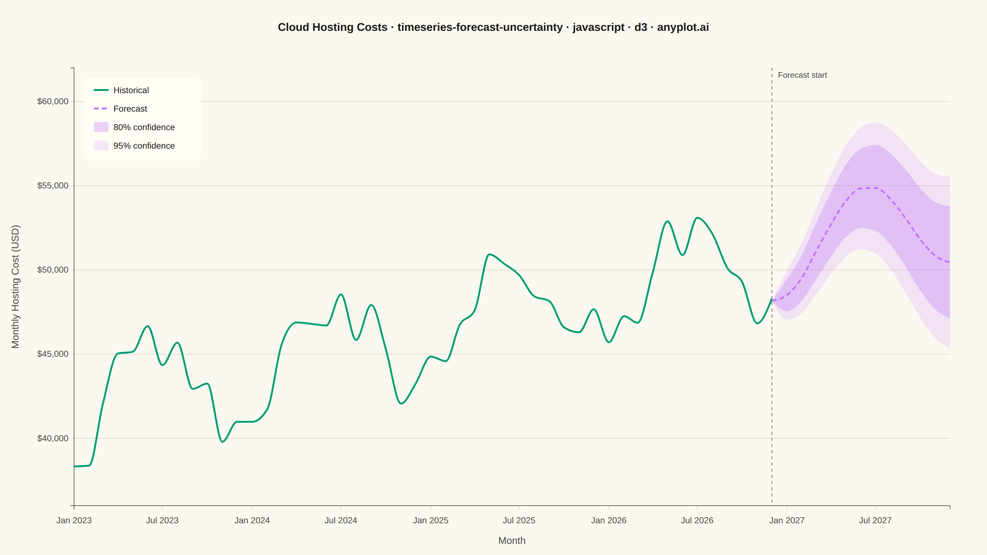
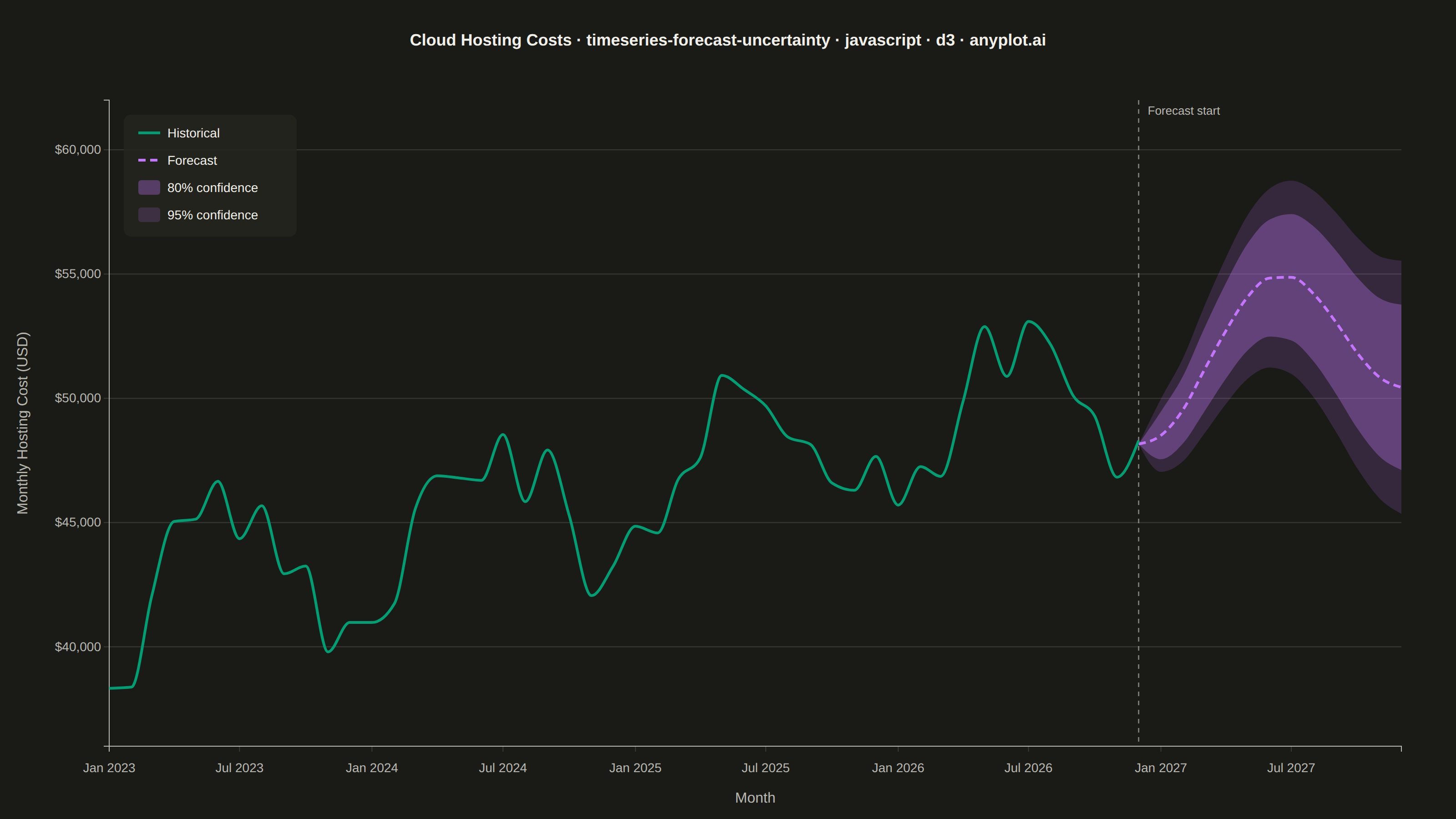
The same plot in 14 other libraries — JavaScript: Chart.js, Apache ECharts, Highcharts, MUI X Charts; Python: Altair, Bokeh, lets-plot, Matplotlib, Plotly, plotnine, Pygal, Seaborn; R: ggplot2; Julia: Makie.jl. Compare all 15 side by side: Time Series Forecast with Uncertainty Band in Python, R, Julia and JavaScript.
A time series plot that displays historical observed data followed by a forecast projection with confidence intervals or uncertainty bands. The plot clearly distinguishes between the historical period and the forecast period using a vertical line marker, with shaded bands representing different confidence levels (typically 80% and 95%). This visualization is essential for communicating prediction uncertainty in forecasting applications, helping stakeholders understand both the expected values and the range of possible outcomes.
// anyplot.ai
// timeseries-forecast-uncertainty: Time Series Forecast with Uncertainty Band
// Library: d3 7.9.0 | JavaScript 22.23.2
// Quality: 89/100 | Created: 2026-09-02

const t = window.ANYPLOT_TOKENS;
const { width, height } = window.ANYPLOT_SIZE;
const margin = { top: 110, right: 60, bottom: 80, left: 120 };
const iw = width - margin.left - margin.right;
const ih = height - margin.top - margin.bottom;

// --- Data (in-memory, deterministic) ----------------------------------------
// Monthly cloud-hosting spend: 4 years (48 months) of observed history plus a
// 12-month forecast. The forecast series starts one month before its horizon
// begins (index 47) so the historical and forecast lines join seamlessly.
let seed = 20260902;
function lcg() {
  seed = (seed * 1664525 + 1013904223) % 4294967296;
  return seed / 4294967296;
}
function gaussian() {
  // Box-Muller, using the deterministic LCG above.
  const u1 = Math.max(lcg(), 1e-9);
  const u2 = lcg();
  return Math.sqrt(-2 * Math.log(u1)) * Math.cos(2 * Math.PI * u2);
}

const historicalMonths = 48;
const forecastHorizon = 12;
const totalMonths = historicalMonths + forecastHorizon;
const forecastStart = historicalMonths - 1; // last historical month == first forecast month

const dates = Array.from({ length: totalMonths }, (_, i) => new Date(2023, i, 1));

const base = 42000; // USD / month
const monthlyGrowth = 190;
const seasonalAmplitude = 2800;
const noiseStd = 1100;
const sigmaBase = 750; // per-step forecast-uncertainty growth

function centralValue(i) {
  return base + monthlyGrowth * i + seasonalAmplitude * Math.sin((2 * Math.PI * i) / 12 - 1.2);
}

const data = dates.map((date, i) => {
  const central = centralValue(i);
  const row = { date, actual: null, forecast: null, lower_80: null, upper_80: null, lower_95: null, upper_95: null };
  if (i <= historicalMonths - 1) {
    row.actual = Math.round(central + gaussian() * noiseStd);
  }
  if (i >= forecastStart) {
    const h = i - forecastStart;
    const sigma = sigmaBase * Math.sqrt(h);
    row.forecast = Math.round(central);
    row.lower_80 = Math.round(central - 1.2816 * sigma);
    row.upper_80 = Math.round(central + 1.2816 * sigma);
    row.lower_95 = Math.round(central - 1.96 * sigma);
    row.upper_95 = Math.round(central + 1.96 * sigma);
  }
  return row;
});

// --- Colors ------------------------------------------------------------------
const historicalColor = t.palette[0]; // brand green — observed data
const forecastColor = t.palette[1]; // canonical position 2 — prediction + uncertainty family

// --- SVG mount -----------------------------------------------------------------
const svg = d3.select("#container").append("svg").attr("width", width).attr("height", height);
const g = svg.append("g").attr("transform", `translate(${margin.left},${margin.top})`);

// --- Scales --------------------------------------------------------------------
const x = d3.scaleTime().domain(d3.extent(dates)).range([0, iw]);
const values = data.flatMap((d) => [d.actual, d.forecast, d.lower_95, d.upper_95]).filter((v) => v != null);
const y = d3
  .scaleLinear()
  .domain([d3.min(values) * 0.97, d3.max(values) * 1.03])
  .nice()
  .range([ih, 0]);

// --- Gridlines -------------------------------------------------------------
g.append("g")
  .attr("class", "grid")
  .call(d3.axisLeft(y).ticks(6).tickSize(-iw).tickFormat(""))
  .call((sel) => sel.select(".domain").remove())
  .selectAll("line")
  .attr("stroke", t.grid);

// --- Confidence bands (95% wider + lighter underneath, 80% narrower + darker on top) ---
const area95 = d3
  .area()
  .defined((d) => d.lower_95 != null)
  .x((d) => x(d.date))
  .y0((d) => y(d.lower_95))
  .y1((d) => y(d.upper_95))
  .curve(d3.curveMonotoneX);

const area80 = d3
  .area()
  .defined((d) => d.lower_80 != null)
  .x((d) => x(d.date))
  .y0((d) => y(d.lower_80))
  .y1((d) => y(d.upper_80))
  .curve(d3.curveMonotoneX);

g.append("path").datum(data).attr("d", area95).attr("fill", forecastColor).attr("fill-opacity", 0.16).attr("stroke", "none");
g.append("path").datum(data).attr("d", area80).attr("fill", forecastColor).attr("fill-opacity", 0.32).attr("stroke", "none");

// --- Axes ------------------------------------------------------------------
const xAxis = g
  .append("g")
  .attr("transform", `translate(0,${ih})`)
  .call(d3.axisBottom(x).ticks(d3.timeMonth.every(6)).tickFormat(d3.timeFormat("%b %Y")));
const yAxis = g.append("g").call(d3.axisLeft(y).ticks(6).tickFormat(d3.format("$,.0f")));

for (const ax of [xAxis, yAxis]) {
  ax.selectAll("text").attr("fill", t.inkSoft).style("font-size", "14px");
  ax.selectAll("line").attr("stroke", t.grid);
  ax.select(".domain").attr("stroke", t.inkSoft);
}
xAxis.selectAll("text").attr("dy", "1.4em");

g.append("text")
  .attr("x", iw / 2)
  .attr("y", ih + 62)
  .attr("text-anchor", "middle")
  .attr("fill", t.inkSoft)
  .style("font-size", "16px")
  .text("Month");

g.append("text")
  .attr("transform", "rotate(-90)")
  .attr("x", -ih / 2)
  .attr("y", -90)
  .attr("text-anchor", "middle")
  .attr("fill", t.inkSoft)
  .style("font-size", "16px")
  .text("Monthly Hosting Cost (USD)");

// --- Forecast-start marker ---------------------------------------------------
const markerX = x(dates[forecastStart]);
g.append("line")
  .attr("x1", markerX)
  .attr("x2", markerX)
  .attr("y1", 0)
  .attr("y2", ih)
  .attr("stroke", t.inkSoft)
  .attr("stroke-width", 1.5)
  .attr("stroke-dasharray", "5,5")
  .attr("opacity", 0.6);

g.append("text")
  .attr("x", markerX + 10)
  .attr("y", 16)
  .attr("fill", t.inkSoft)
  .style("font-size", "13px")
  .text("Forecast start");

// --- Lines: solid historical, dashed forecast (drawn above the bands) --------
const lineActual = d3
  .line()
  .defined((d) => d.actual != null)
  .x((d) => x(d.date))
  .y((d) => y(d.actual))
  .curve(d3.curveMonotoneX);

const lineForecast = d3
  .line()
  .defined((d) => d.forecast != null)
  .x((d) => x(d.date))
  .y((d) => y(d.forecast))
  .curve(d3.curveMonotoneX);

g.append("path").datum(data).attr("d", lineForecast).attr("fill", "none").attr("stroke", forecastColor).attr("stroke-width", 3).attr("stroke-dasharray", "8,5");
g.append("path").datum(data).attr("d", lineActual).attr("fill", "none").attr("stroke", historicalColor).attr("stroke-width", 3);

// --- Legend (floating card, top-left of the plot area) -----------------------
const legendItems = [
  { label: "Historical", type: "line", color: historicalColor, dash: null },
  { label: "Forecast", type: "line", color: forecastColor, dash: "8,5" },
  { label: "80% confidence", type: "swatch", color: forecastColor, opacity: 0.32 },
  { label: "95% confidence", type: "swatch", color: forecastColor, opacity: 0.16 },
];

const legend = g.append("g").attr("transform", `translate(16, 16)`);
legend
  .append("rect")
  .attr("width", 190)
  .attr("height", legendItems.length * 30 + 14)
  .attr("rx", 8)
  .attr("fill", t.elevatedBg)
  .attr("opacity", 0.92);

const legendRows = legend
  .selectAll("g.row")
  .data(legendItems)
  .join("g")
  .attr("class", "row")
  .attr("transform", (_, i) => `translate(16, ${20 + i * 30})`);

legendRows.each(function (d) {
  const row = d3.select(this);
  if (d.type === "line") {
    row
      .append("line")
      .attr("x1", 0)
      .attr("x2", 24)
      .attr("y1", 0)
      .attr("y2", 0)
      .attr("stroke", d.color)
      .attr("stroke-width", 3)
      .attr("stroke-dasharray", d.dash);
  } else {
    row.append("rect").attr("x", 0).attr("y", -8).attr("width", 24).attr("height", 16).attr("rx", 3).attr("fill", d.color).attr("fill-opacity", d.opacity);
  }
  row.append("text").attr("x", 32).attr("y", 5).attr("fill", t.ink).style("font-size", "14px").text(d.label);
});

// --- Title -------------------------------------------------------------------
const title = "Cloud Hosting Costs · timeseries-forecast-uncertainty · javascript · d3 · anyplot.ai";
const titleFontSize = Math.max(14, Math.round(22 * Math.min(1, 67 / title.length)));
svg
  .append("text")
  .attr("x", width / 2)
  .attr("y", 50)
  .attr("text-anchor", "middle")
  .attr("fill", t.ink)
  .style("font-size", `${titleFontSize}px`)
  .style("font-weight", "600")
  .text(title);
Runnable source as JSON, for any HTTP client: https://api.anyplot.ai/specs/timeseries-forecast-uncertainty/d3/code. Any spec id and library id listed in llms-full.txt fit the same URL shape; every URL below is complete and callable.
{
  "spec_id": "timeseries-forecast-uncertainty",
  "language": "javascript",
  "library": "d3",
  "page": "https://anyplot.ai/timeseries-forecast-uncertainty/javascript/d3",
  "hub": "https://anyplot.ai/timeseries-forecast-uncertainty",
  "code_json": "https://api.anyplot.ai/specs/timeseries-forecast-uncertainty/d3/code",
  "spec_json": "https://api.anyplot.ai/specs/timeseries-forecast-uncertainty",
  "render_light_png": "https://storage.googleapis.com/anyplot-images/plots/timeseries-forecast-uncertainty/javascript/d3/plot-light.png",
  "render_dark_png": "https://storage.googleapis.com/anyplot-images/plots/timeseries-forecast-uncertainty/javascript/d3/plot-dark.png",
  "interactive_light_html": "https://storage.googleapis.com/anyplot-images/plots/timeseries-forecast-uncertainty/javascript/d3/plot-light.html",
  "interactive_dark_html": "https://storage.googleapis.com/anyplot-images/plots/timeseries-forecast-uncertainty/javascript/d3/plot-dark.html",
  "quality_score": 89.0,
  "license": "MIT",
  "guide": "https://anyplot.ai/llms.txt"
}
Part of Time Series Forecast with Uncertainty Band on anyplot.ai.