The same plot in 14 other libraries — Python: Altair, Bokeh, lets-plot, Matplotlib, Plotly, plotnine, Pygal, Seaborn; R: ggplot2; JavaScript: Chart.js, D3.js, Apache ECharts, Highcharts, MUI X Charts. Compare all 15 side by side: Violin Plot with Overlaid Swarm Points in Python, R, Julia and JavaScript.
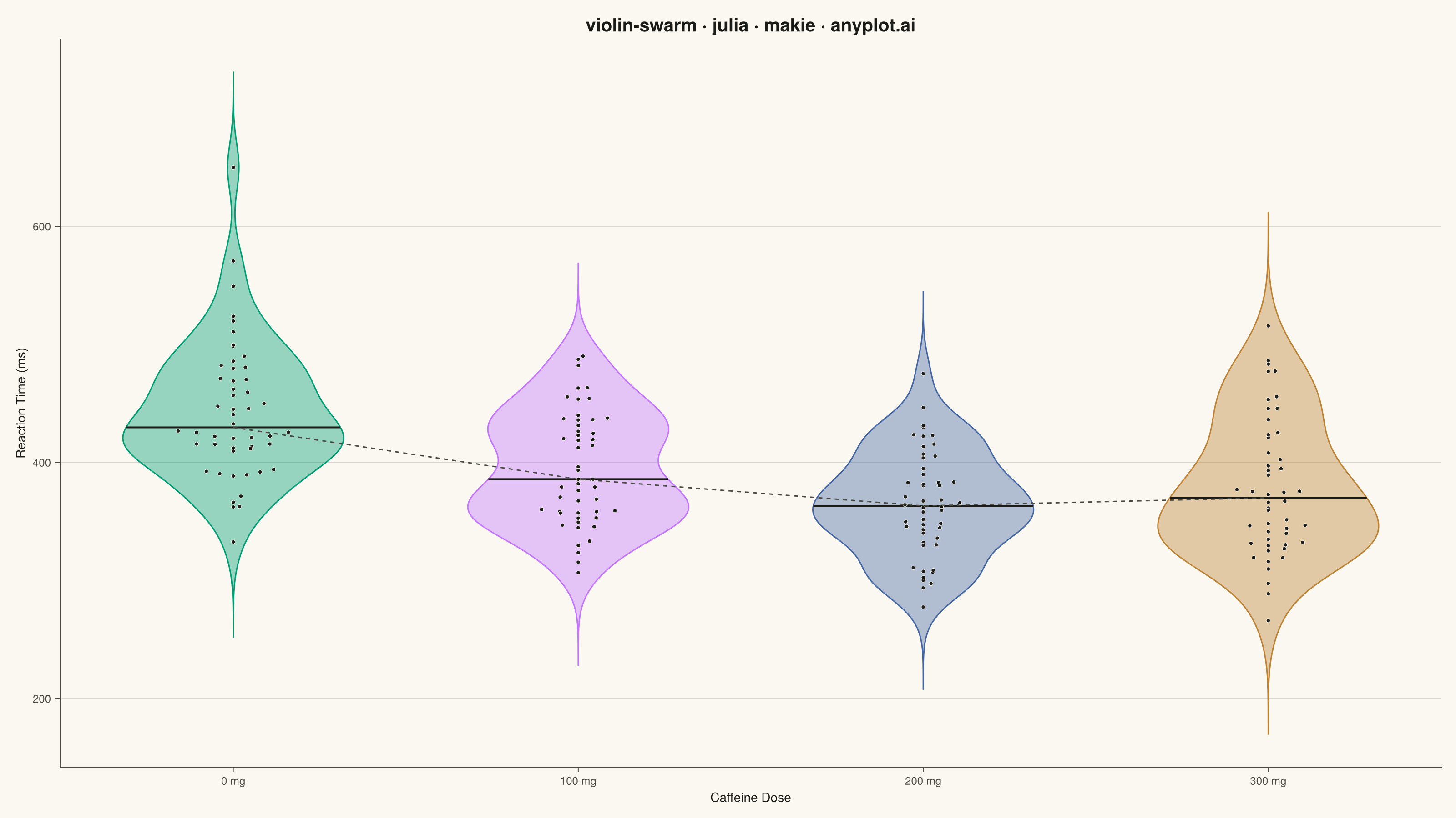
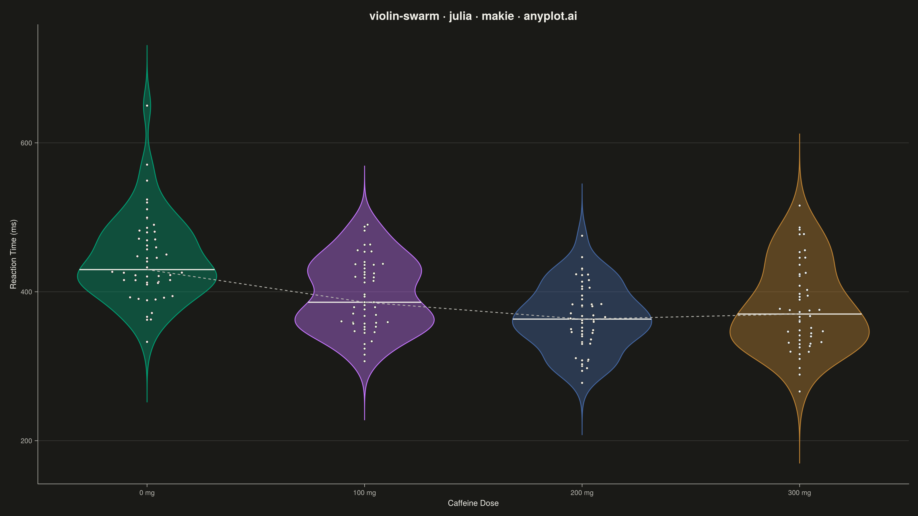
A violin plot with individual data points overlaid as a swarm plot, combining smooth kernel density estimation with raw data visibility. The violin shape shows the distribution density while the swarm points reveal actual observations, enabling viewers to see both the overall distribution pattern and individual data values simultaneously. This hybrid approach provides maximum transparency, showing exactly how many observations exist at each level while maintaining the smooth distribution visualization.
# anyplot.ai
# violin-swarm: Violin Plot with Overlaid Swarm Points
# Library: makie 0.21.9 | Julia 1.11.9
# Quality: 85/100 | Created: 2026-09-02

using CairoMakie
using Colors
using Random
using Statistics

Random.seed!(42)

# Theme tokens (see prompts/default-style-guide.md "Theme-adaptive Chrome")
const THEME    = get(ENV, "ANYPLOT_THEME", "light")
const PAGE_BG  = THEME == "light" ? colorant"#FAF8F1" : colorant"#1A1A17"
const INK      = THEME == "light" ? colorant"#1A1A17" : colorant"#F0EFE8"
const INK_SOFT = THEME == "light" ? colorant"#4A4A44" : colorant"#B8B7B0"

# Imprint categorical palette — 8 hues, theme-independent, hybrid-v3 sort
const IMPRINT_PALETTE = [
    colorant"#009E73",  # 1 — brand green
    colorant"#C475FD",  # 2 — lavender
    colorant"#4467A3",  # 3 — blue
    colorant"#BD8233",  # 4 — ochre
]

# Data — reaction time (ms) across 4 caffeine dosage groups, 50 trials each.
# Right-skewed noise mimics the long slow-trial tail typical of RT data, and
# the 300 mg group's uptick models overstimulation jitter past the optimum.
const DOSE_LABELS = ["0 mg", "100 mg", "200 mg", "300 mg"]
const BASELINE_MS = [430.0, 388.0, 356.0, 368.0]
const SPREAD_MS   = [46.0, 40.0, 34.0, 50.0]
const N_PER_GROUP = 50

dose_idx         = Int[]
reaction_time_ms = Float64[]
for (i, (base, spread)) in enumerate(zip(BASELINE_MS, SPREAD_MS))
    noise      = randn(N_PER_GROUP)
    right_tail = 0.35 .* spread .* max.(noise, 0.0)
    trials     = clamp.(base .+ spread .* noise .+ right_tail, 180.0, 650.0)
    append!(reaction_time_ms, trials)
    append!(dose_idx, fill(i, N_PER_GROUP))
end

# Gaussian KDE — approximates the same density curve Makie's violin! draws,
# so the swarm's allowed spread can be tied to the violin's actual local
# width instead of raw histogram counts.
function kde_density(values, x, bandwidth)
    z = (x .- values) ./ bandwidth
    return sum(exp.(-0.5 .* z .^ 2)) / (length(values) * bandwidth * sqrt(2π))
end

# Beeswarm layout — bin each category's trials by value, then stack points
# alternating left/right of center within a bin. Each bin's half-width is
# the local KDE density (relative to the category's peak density) scaled to
# max_half_width, so the allowed spread narrows exactly where the violin
# body narrows and points never escape the outline.
function beeswarm_offsets(values, max_half_width, n_bins)
    n      = length(values)
    lo, hi = minimum(values), maximum(values)
    # Silverman's rule of thumb bandwidth, inlined (single call site).
    sigma  = min(std(values), (quantile(values, 0.75) - quantile(values, 0.25)) / 1.34)
    bw     = 0.9 * sigma * n^(-0.2)

    bin_edges   = range(lo, hi, length = n_bins + 1)
    bin_centers = (bin_edges[1:(end - 1)] .+ bin_edges[2:end]) ./ 2
    bin_density = [kde_density(values, c, bw) for c in bin_centers]
    peak        = maximum(bin_density)
    bin_width   = max_half_width .* bin_density ./ peak

    offsets     = zeros(Float64, n)
    span        = hi - lo
    slot_of_bin = zeros(Int, n_bins)
    for idx in sortperm(values)
        b = span > 0 ? clamp(floor(Int, (values[idx] - lo) / span * n_bins), 0, n_bins - 1) + 1 : 1
        slot = slot_of_bin[b]
        slot_of_bin[b] += 1
        side      = isodd(slot) ? 1 : -1
        magnitude = slot == 0 ? 0.0 : ceil(slot / 2)
        step      = bin_width[b] / 6.0
        offsets[idx] = clamp(side * magnitude * step, -bin_width[b], bin_width[b])
    end
    return offsets
end

const VIOLIN_WIDTH     = 0.8
const SWARM_HALF_WIDTH = 0.32
const N_BINS           = 40

swarm_offset = zeros(Float64, length(reaction_time_ms))
for i in eachindex(DOSE_LABELS)
    mask = dose_idx .== i
    swarm_offset[mask] = beeswarm_offsets(reaction_time_ms[mask], SWARM_HALF_WIDTH, N_BINS)
end
swarm_x = Float64.(dose_idx) .+ swarm_offset

# Plot — see default-style-guide.md "Visual Sizing Defaults" for canvas + sizing values
title_str = "violin-swarm · julia · makie · anyplot.ai"

fig = Figure(
    resolution      = (1600, 900),
    fontsize        = 14,
    backgroundcolor = PAGE_BG,
)

ax = Axis(
    fig[1, 1];
    title             = title_str,
    titlesize         = 20,
    titlecolor        = INK,
    xlabel            = "Caffeine Dose",
    ylabel            = "Reaction Time (ms)",
    xlabelsize        = 14,
    ylabelsize        = 14,
    xlabelcolor       = INK,
    ylabelcolor       = INK,
    xticklabelsize    = 12,
    yticklabelsize    = 12,
    xticklabelcolor   = INK_SOFT,
    yticklabelcolor   = INK_SOFT,
    xtickcolor        = INK_SOFT,
    ytickcolor        = INK_SOFT,
    backgroundcolor   = PAGE_BG,
    topspinevisible   = false,
    rightspinevisible = false,
    leftspinecolor    = INK_SOFT,
    bottomspinecolor  = INK_SOFT,
    xgridvisible      = false,
    ygridcolor        = RGBAf(INK.r, INK.g, INK.b, 0.15),
    yminorgridvisible = false,
    xminorgridvisible = false,
    xticks            = (1:length(DOSE_LABELS), DOSE_LABELS),
)

# Translucent violins (alpha 0.4) so the swarm underneath stays legible.
# show_median draws Makie's native per-violin median line — a built-in
# violin! feature (not a manual overlay) that anchors each group's center.
for (i, col) in enumerate(IMPRINT_PALETTE)
    mask = dose_idx .== i
    violin!(ax, dose_idx[mask], reaction_time_ms[mask];
        color           = (col, 0.4),
        strokewidth     = 1.5,
        strokecolor     = col,
        width           = VIOLIN_WIDTH,
        show_median     = true,
        mediancolor     = INK,
        medianlinewidth = 2.0,
    )
end

# Dashed trend line through each group's median sharpens the inverted-U
# dose-response story (reaction time drops, then rises again at 300 mg).
medians_ms = [median(reaction_time_ms[dose_idx .== i]) for i in eachindex(DOSE_LABELS)]
lines!(ax, 1:length(DOSE_LABELS), medians_ms;
    color     = INK_SOFT,
    linewidth = 1.5,
    linestyle = :dash,
)

# Ink-colored swarm points contrast against every translucent violin hue
scatter!(ax, swarm_x, reaction_time_ms;
    color       = INK,
    markersize  = 6,
    strokewidth = 0.5,
    strokecolor = PAGE_BG,
)

# Save
save("plot-$(THEME).png", fig; px_per_unit = 2)
Runnable source as JSON, for any HTTP client: https://api.anyplot.ai/specs/violin-swarm/makie/code. Any spec id and library id listed in llms-full.txt fit the same URL shape; every URL below is complete and callable.
{
  "spec_id": "violin-swarm",
  "language": "julia",
  "library": "makie",
  "page": "https://anyplot.ai/violin-swarm/julia/makie",
  "hub": "https://anyplot.ai/violin-swarm",
  "code_json": "https://api.anyplot.ai/specs/violin-swarm/makie/code",
  "spec_json": "https://api.anyplot.ai/specs/violin-swarm",
  "render_light_png": "https://storage.googleapis.com/anyplot-images/plots/violin-swarm/julia/makie/plot-light.png",
  "render_dark_png": "https://storage.googleapis.com/anyplot-images/plots/violin-swarm/julia/makie/plot-dark.png",
  "quality_score": 85.0,
  "license": "MIT",
  "guide": "https://anyplot.ai/llms.txt"
}
Part of Violin Plot with Overlaid Swarm Points on anyplot.ai.