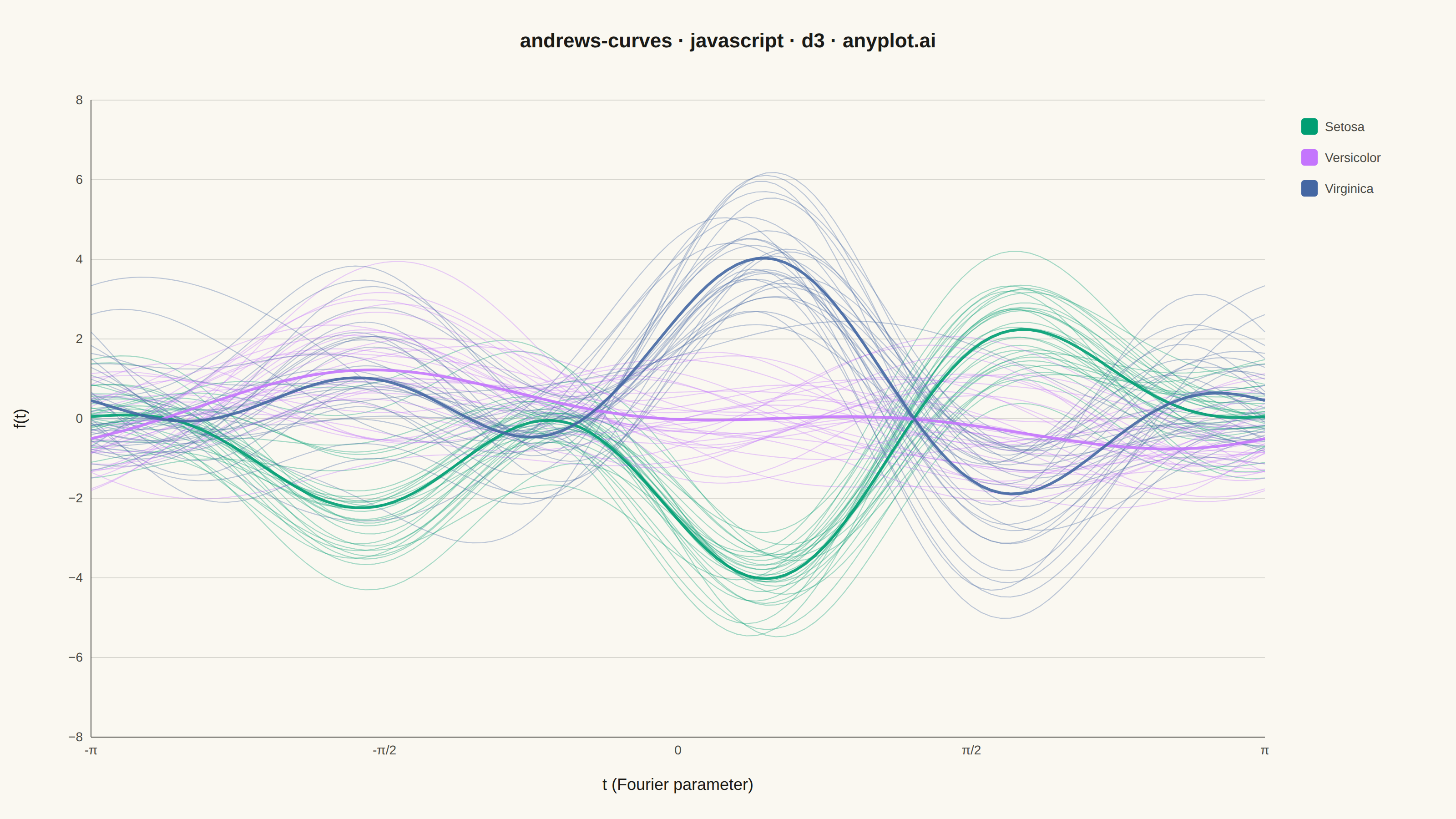
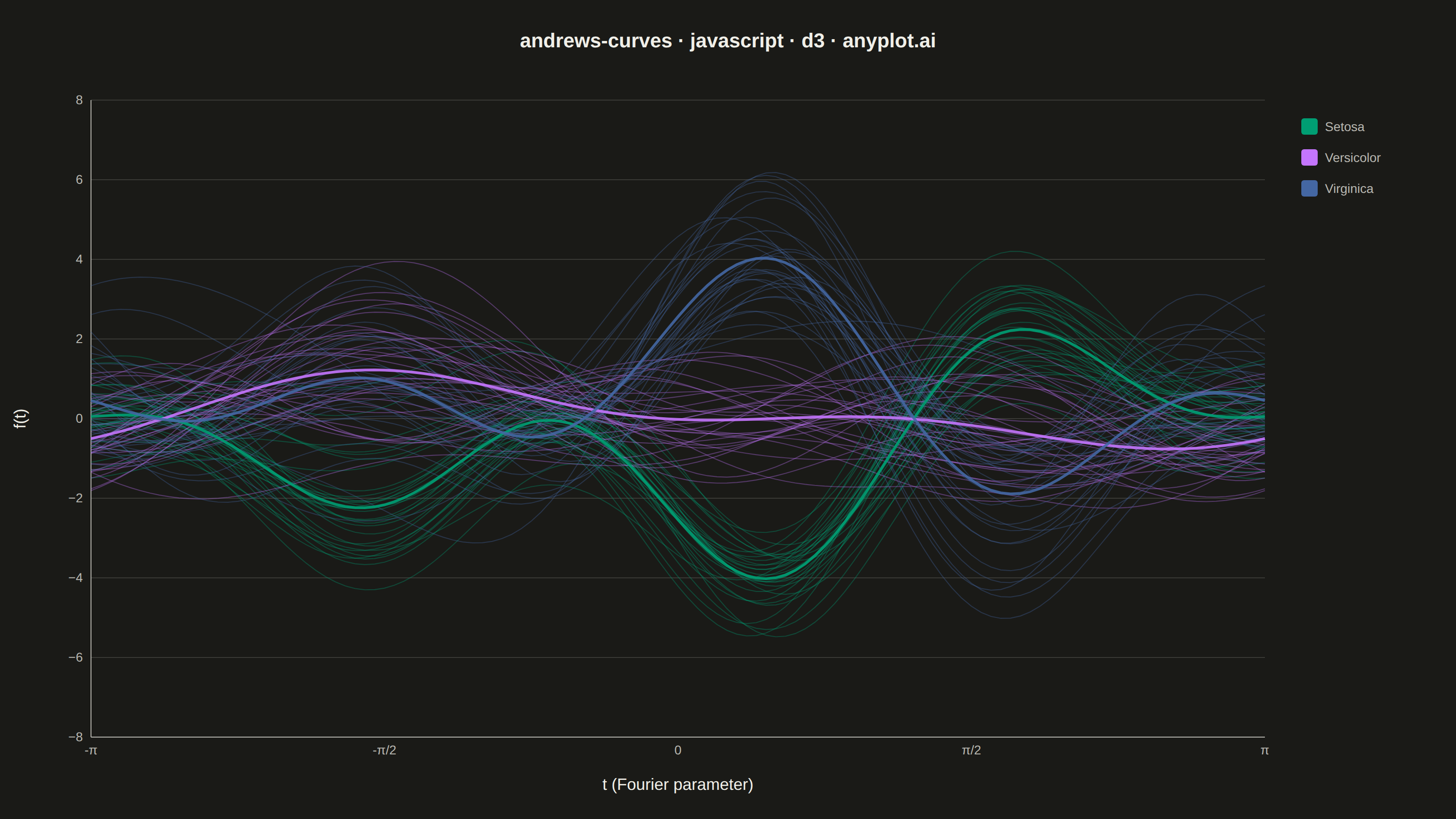
The same plot in 14 other libraries — JavaScript: Chart.js, Apache ECharts, Highcharts, MUI X Charts; Python: Altair, Bokeh, lets-plot, Matplotlib, Plotly, plotnine, Pygal, Seaborn; R: ggplot2; Julia: Makie.jl. Compare all 15 side by side: Andrews Curves for Multivariate Data in Python, R, Julia and JavaScript.
Andrews curves visualization transforms multivariate observations into smooth Fourier series curves. Each data point is represented as a continuous function where variable values become coefficients in a Fourier expansion, producing distinctive wave patterns. This technique enables visual comparison of multivariate patterns, cluster identification, and outlier detection—observations with similar values across variables produce similar curves, while outliers appear as distinctly different patterns.
// anyplot.ai
// andrews-curves: Andrews Curves for Multivariate Data
// Library: d3 7.9.0 | JavaScript 22.23.2
// Quality: 92/100 | Created: 2026-09-02

const t = window.ANYPLOT_TOKENS;
const { width, height } = window.ANYPLOT_SIZE;
const margin = { top: 110, right: 210, bottom: 90, left: 100 };
const iw = width - margin.left - margin.right;
const ih = height - margin.top - margin.bottom;

// --- Data: synthetic iris-like measurements (6 variables, 3 species) -------
// Deterministic LCG (the browser has no seeded Math.random) drives a
// Box-Muller transform so each species clusters around realistic means.
let seed = 42;
function lcg() {
  seed = (seed * 1103515245 + 12345) % 2147483648;
  return seed / 2147483648;
}
function gaussian(mean, std) {
  const u1 = lcg() || 1e-9;
  const u2 = lcg();
  const z = Math.sqrt(-2 * Math.log(u1)) * Math.cos(2 * Math.PI * u2);
  return mean + z * std;
}

// 6 variables per observation: the 4 classic iris measurements plus 2 derived
// area measurements (sepal_area, petal_area), giving the Andrews expansion
// fuller use of its 4-8 recommended dimensionality.
const species = [
  {
    name: "setosa",
    n: 30,
    means: [5.0, 3.4, 1.5, 0.2, 17.0, 0.3],
    stds: [0.35, 0.38, 0.17, 0.11, 1.8, 0.15],
  },
  {
    name: "versicolor",
    n: 30,
    means: [5.9, 2.8, 4.3, 1.3, 16.5, 5.6],
    stds: [0.52, 0.31, 0.47, 0.2, 2.2, 1.0],
  },
  {
    name: "virginica",
    n: 30,
    means: [6.6, 3.0, 5.6, 2.0, 19.8, 11.2],
    stds: [0.64, 0.32, 0.55, 0.27, 2.6, 1.8],
  },
];

const observations = [];
for (const sp of species) {
  for (let i = 0; i < sp.n; i++) {
    observations.push({
      species: sp.name,
      values: sp.means.map((m, j) => gaussian(m, sp.stds[j])),
    });
  }
}

// Standardize each variable (z-score) so no single measurement dominates
const dims = observations[0].values.length;
for (let j = 0; j < dims; j++) {
  const col = observations.map((o) => o.values[j]);
  const mean = d3.mean(col);
  const std = d3.deviation(col);
  observations.forEach((o) => (o.values[j] = (o.values[j] - mean) / std));
}

// --- Andrews curve: x1/sqrt(2) + x2 sin(t) + x3 cos(t) + x4 sin(2t) + ... --
// General Fourier expansion so any number of standardized variables (here 6)
// contributes alternating sin/cos terms at increasing frequency.
function andrews(tt, v) {
  let f = v[0] / Math.SQRT2;
  for (let k = 1; k < v.length; k++) {
    const freq = Math.ceil(k / 2);
    f += k % 2 === 1 ? v[k] * Math.sin(freq * tt) : v[k] * Math.cos(freq * tt);
  }
  return f;
}

const N_SAMPLES = 120;
const tSamples = d3.range(N_SAMPLES + 1).map((i) => -Math.PI + (2 * Math.PI * i) / N_SAMPLES);

const curves = observations.map((o) => ({
  species: o.species,
  points: tSamples.map((tt) => ({ t: tt, value: andrews(tt, o.values) })),
}));

// Per-species mean curve (Andrews is linear in v, so this is the curve of the
// mean vector) drawn bolder on top, giving the dense central overlap a clear
// visual-hierarchy anchor beyond color alone.
const meanCurves = species.map((sp) => {
  const spValues = observations.filter((o) => o.species === sp.name).map((o) => o.values);
  const meanValues = d3.range(dims).map((j) => d3.mean(spValues, (v) => v[j]));
  return {
    species: sp.name,
    points: tSamples.map((tt) => ({ t: tt, value: andrews(tt, meanValues) })),
  };
});

const yExtent = d3.extent(curves.flatMap((c) => c.points.map((p) => p.value)));
const yPad = (yExtent[1] - yExtent[0]) * 0.08;

// --- SVG mount ---------------------------------------------------------------
const svg = d3.select("#container").append("svg").attr("width", width).attr("height", height);
const g = svg.append("g").attr("transform", `translate(${margin.left},${margin.top})`);

// --- Scales -------------------------------------------------------------------
const x = d3.scaleLinear().domain([-Math.PI, Math.PI]).range([0, iw]);
const y = d3
  .scaleLinear()
  .domain([yExtent[0] - yPad, yExtent[1] + yPad])
  .nice()
  .range([ih, 0]);
const color = d3
  .scaleOrdinal()
  .domain(species.map((s) => s.name))
  .range(t.palette);

// --- Gridlines (y-axis only) -------------------------------------------------
g.append("g")
  .selectAll("line")
  .data(y.ticks(6))
  .join("line")
  .attr("x1", 0)
  .attr("x2", iw)
  .attr("y1", (d) => y(d))
  .attr("y2", (d) => y(d))
  .attr("stroke", t.grid)
  .attr("stroke-width", 1);

// --- Axes -----------------------------------------------------------------
const piTicks = [-Math.PI, -Math.PI / 2, 0, Math.PI / 2, Math.PI];
const piLabels = ["-π", "-π/2", "0", "π/2", "π"];
const xAxis = g
  .append("g")
  .attr("transform", `translate(0,${ih})`)
  .call(
    d3
      .axisBottom(x)
      .tickValues(piTicks)
      .tickFormat((d, i) => piLabels[i])
      .tickSizeOuter(0)
  );
const yAxis = g.append("g").call(d3.axisLeft(y).ticks(6).tickSizeOuter(0));

for (const ax of [xAxis, yAxis]) {
  ax.selectAll("text").attr("fill", t.inkSoft).style("font-size", "14px");
  ax.select(".domain").attr("stroke", t.inkSoft);
}
xAxis.selectAll(".tick line").remove();
yAxis.selectAll(".tick line").remove();

// --- Axis labels -------------------------------------------------------------
g.append("text")
  .attr("x", iw / 2)
  .attr("y", ih + 58)
  .attr("text-anchor", "middle")
  .attr("fill", t.ink)
  .style("font-size", "18px")
  .text("t (Fourier parameter)");

g.append("text")
  .attr("transform", "rotate(-90)")
  .attr("x", -ih / 2)
  .attr("y", -72)
  .attr("text-anchor", "middle")
  .attr("fill", t.ink)
  .style("font-size", "18px")
  .text("f(t)");

// --- Curves --------------------------------------------------------------
const line = d3
  .line()
  .x((d) => x(d.t))
  .y((d) => y(d.value));

g.selectAll("path.curve")
  .data(curves)
  .join("path")
  .attr("class", "curve")
  .attr("d", (d) => line(d.points))
  .attr("fill", "none")
  .attr("stroke", (d) => color(d.species))
  .attr("stroke-width", 1.1)
  .attr("stroke-opacity", 0.35);

// Bolder mean curves on top, one per species, for visual hierarchy.
g.selectAll("path.mean-curve")
  .data(meanCurves)
  .join("path")
  .attr("class", "mean-curve")
  .attr("d", (d) => line(d.points))
  .attr("fill", "none")
  .attr("stroke", (d) => color(d.species))
  .attr("stroke-width", 3)
  .attr("stroke-opacity", 0.9);

// --- Legend ------------------------------------------------------------------
const legend = svg
  .append("g")
  .attr("transform", `translate(${margin.left + iw + 40},${margin.top + 20})`);
species.forEach((sp, i) => {
  const row = legend.append("g").attr("transform", `translate(0,${i * 34})`);
  row
    .append("rect")
    .attr("width", 18)
    .attr("height", 18)
    .attr("rx", 3)
    .attr("fill", color(sp.name));
  row
    .append("text")
    .attr("x", 26)
    .attr("y", 14)
    .attr("fill", t.inkSoft)
    .style("font-size", "14px")
    .text(sp.name[0].toUpperCase() + sp.name.slice(1));
});

// --- Title ---------------------------------------------------------------------
svg
  .append("text")
  .attr("x", width / 2)
  .attr("y", 52)
  .attr("text-anchor", "middle")
  .attr("fill", t.ink)
  .style("font-size", "22px")
  .style("font-weight", "600")
  .text("andrews-curves · javascript · d3 · anyplot.ai");
Runnable source as JSON, for any HTTP client: https://api.anyplot.ai/specs/andrews-curves/d3/code. Any spec id and library id listed in llms-full.txt fit the same URL shape; every URL below is complete and callable.
{
  "spec_id": "andrews-curves",
  "language": "javascript",
  "library": "d3",
  "page": "https://anyplot.ai/andrews-curves/javascript/d3",
  "hub": "https://anyplot.ai/andrews-curves",
  "code_json": "https://api.anyplot.ai/specs/andrews-curves/d3/code",
  "spec_json": "https://api.anyplot.ai/specs/andrews-curves",
  "render_light_png": "https://storage.googleapis.com/anyplot-images/plots/andrews-curves/javascript/d3/plot-light.png",
  "render_dark_png": "https://storage.googleapis.com/anyplot-images/plots/andrews-curves/javascript/d3/plot-dark.png",
  "interactive_light_html": "https://storage.googleapis.com/anyplot-images/plots/andrews-curves/javascript/d3/plot-light.html",
  "interactive_dark_html": "https://storage.googleapis.com/anyplot-images/plots/andrews-curves/javascript/d3/plot-dark.html",
  "quality_score": 92.0,
  "license": "MIT",
  "guide": "https://anyplot.ai/llms.txt"
}
Part of Andrews Curves for Multivariate Data on anyplot.ai.