The same plot in 14 other libraries — Python: Altair, Bokeh, lets-plot, Matplotlib, Plotly, plotnine, Pygal, Seaborn; Julia: Makie.jl; JavaScript: Chart.js, D3.js, Apache ECharts, Highcharts, MUI X Charts. Compare all 15 side by side: Andrews Curves for Multivariate Data in Python, R, Julia and JavaScript.
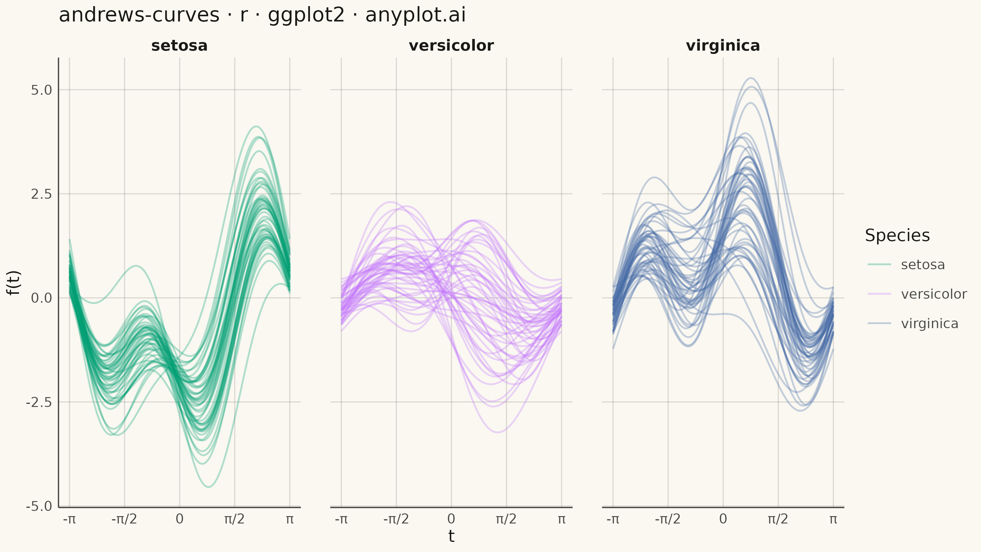
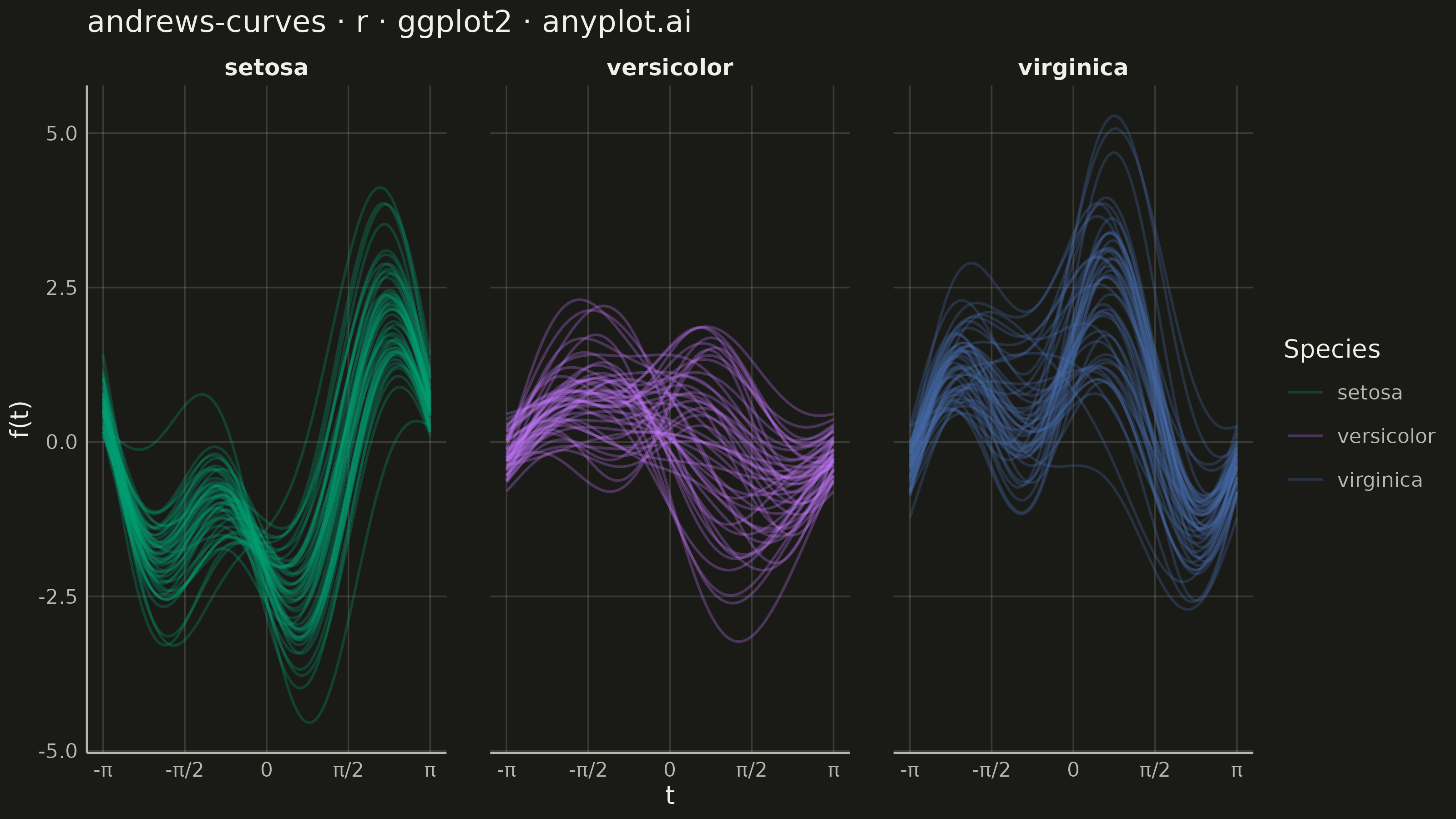
Andrews curves visualization transforms multivariate observations into smooth Fourier series curves. Each data point is represented as a continuous function where variable values become coefficients in a Fourier expansion, producing distinctive wave patterns. This technique enables visual comparison of multivariate patterns, cluster identification, and outlier detection—observations with similar values across variables produce similar curves, while outliers appear as distinctly different patterns.
#' anyplot.ai
#' andrews-curves: Andrews Curves for Multivariate Data
#' Library: ggplot2 3.5.1 | R 4.4.1
#' Quality: 89/100 | Created: 2026-09-02

library(ggplot2)
library(dplyr)
library(tidyr)
library(scales)
library(ragg)

set.seed(42)

# --- Theme tokens -------------------------------------------------------
THEME       <- Sys.getenv("ANYPLOT_THEME", "light")
PAGE_BG     <- if (THEME == "light") "#FAF8F1" else "#1A1A17"
INK         <- if (THEME == "light") "#1A1A17" else "#F0EFE8"
INK_SOFT    <- if (THEME == "light") "#4A4A44" else "#B8B7B0"
GRID_COLOR  <- scales::alpha(INK, 0.15)
IMPRINT_PALETTE <- c("#009E73", "#C475FD", "#4467A3", "#BD8233",
                     "#AE3030", "#2ABCCD", "#954477", "#99B314")

# --- Data -----------------------------------------------------------------
# Iris sepal/petal measurements, z-score normalized so no single dimension
# dominates the Fourier expansion (see specification "Notes").
measurements <- iris %>%
  select(Sepal.Length, Sepal.Width, Petal.Length, Petal.Width) %>%
  scale() %>%
  as.matrix()

species <- iris$Species
n_vars  <- ncol(measurements)

# Andrews curve Fourier basis:
# f(t) = x1/sqrt(2) + x2 sin(t) + x3 cos(t) + x4 sin(2t) + x5 cos(2t) + ...
t_vals <- seq(-pi, pi, length.out = 200)
basis  <- matrix(0, nrow = length(t_vals), ncol = n_vars)
basis[, 1] <- 1 / sqrt(2)
for (k in 2:n_vars) {
  harmonic   <- k %/% 2
  basis[, k] <- if (k %% 2 == 0) sin(harmonic * t_vals) else cos(harmonic * t_vals)
}

curve_values <- measurements %*% t(basis) # observations x t_vals

curves_df <- as.data.frame(curve_values) %>%
  setNames(as.character(t_vals)) %>%
  mutate(obs_id = row_number(), species = species) %>%
  pivot_longer(-c(obs_id, species), names_to = "t", values_to = "f_t") %>%
  mutate(t = as.numeric(t))

# --- Plot -------------------------------------------------------------------
# facet_wrap(~species) splits the overlaid Fourier bands into per-species
# small multiples, so cluster shape is legible even where the pooled overlay
# is densest (t ~= 0) — a ggplot2-idiomatic alternative to a single hairball.
p <- ggplot(curves_df, aes(x = t, y = f_t, group = obs_id, color = species)) +
  geom_line(linewidth = 0.5, alpha = 0.3) +
  facet_wrap(~species, nrow = 1) +
  scale_color_manual(values = IMPRINT_PALETTE[1:3], name = "Species") +
  scale_x_continuous(breaks = c(-pi, -pi / 2, 0, pi / 2, pi),
                      labels = c("-π", "-π/2", "0", "π/2", "π")) +
  labs(title = "andrews-curves · r · ggplot2 · anyplot.ai",
       x = "t", y = "f(t)") +
  theme_minimal(base_size = 8) +
  theme(
    plot.background   = element_rect(fill = PAGE_BG, color = PAGE_BG),
    panel.background  = element_rect(fill = PAGE_BG, color = NA),
    panel.grid.major  = element_line(color = GRID_COLOR, linewidth = 0.3),
    panel.grid.minor  = element_blank(),
    panel.border      = element_blank(),
    panel.spacing     = unit(1.2, "lines"),
    strip.background  = element_blank(),
    strip.text        = element_text(color = INK, size = 9, face = "bold"),
    axis.title        = element_text(color = INK, size = 10),
    axis.text         = element_text(color = INK_SOFT, size = 8),
    axis.line         = element_line(color = INK_SOFT),
    plot.title        = element_text(color = INK, size = 12),
    legend.text       = element_text(color = INK_SOFT, size = 8),
    legend.title      = element_text(color = INK, size = 10),
    legend.background = element_blank(),
    legend.key        = element_blank()
  )

# --- Save -------------------------------------------------------------------
ggsave(
  filename = sprintf("plot-%s.png", THEME),
  plot     = p,
  device   = ragg::agg_png,
  width    = 8,
  height   = 4.5,
  units    = "in",
  dpi      = 400
)
Runnable source as JSON, for any HTTP client: https://api.anyplot.ai/specs/andrews-curves/ggplot2/code. Any spec id and library id listed in llms-full.txt fit the same URL shape; every URL below is complete and callable.
{
  "spec_id": "andrews-curves",
  "language": "r",
  "library": "ggplot2",
  "page": "https://anyplot.ai/andrews-curves/r/ggplot2",
  "hub": "https://anyplot.ai/andrews-curves",
  "code_json": "https://api.anyplot.ai/specs/andrews-curves/ggplot2/code",
  "spec_json": "https://api.anyplot.ai/specs/andrews-curves",
  "render_light_png": "https://storage.googleapis.com/anyplot-images/plots/andrews-curves/r/ggplot2/plot-light.png",
  "render_dark_png": "https://storage.googleapis.com/anyplot-images/plots/andrews-curves/r/ggplot2/plot-dark.png",
  "quality_score": 89.0,
  "license": "MIT",
  "guide": "https://anyplot.ai/llms.txt"
}
Part of Andrews Curves for Multivariate Data on anyplot.ai.