The same plot in 14 other libraries — Python: Altair, Bokeh, Matplotlib, Plotly, plotnine, Pygal, Seaborn; R: ggplot2; Julia: Makie.jl; JavaScript: Chart.js, D3.js, Apache ECharts, Highcharts, MUI X Charts. Compare all 15 side by side: Cumulative Flow Diagram for Workflow Analytics in Python, R, Julia and JavaScript.
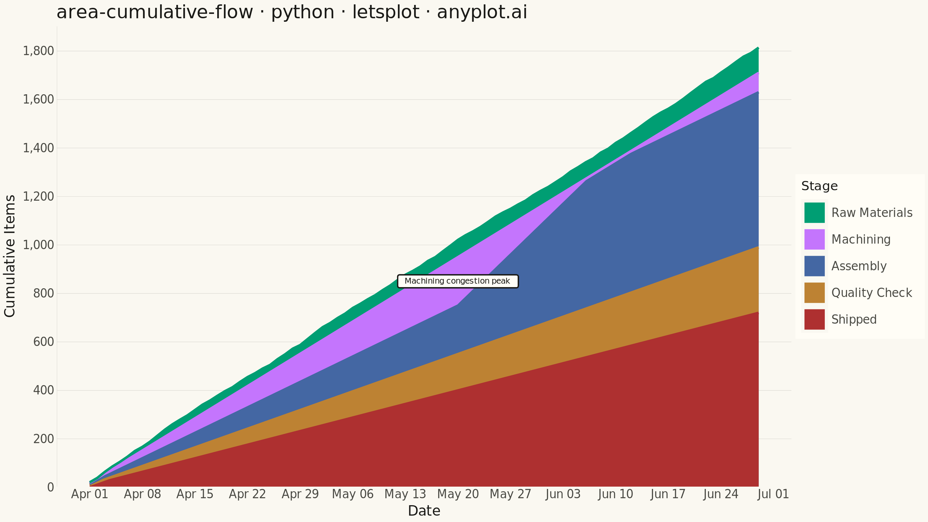
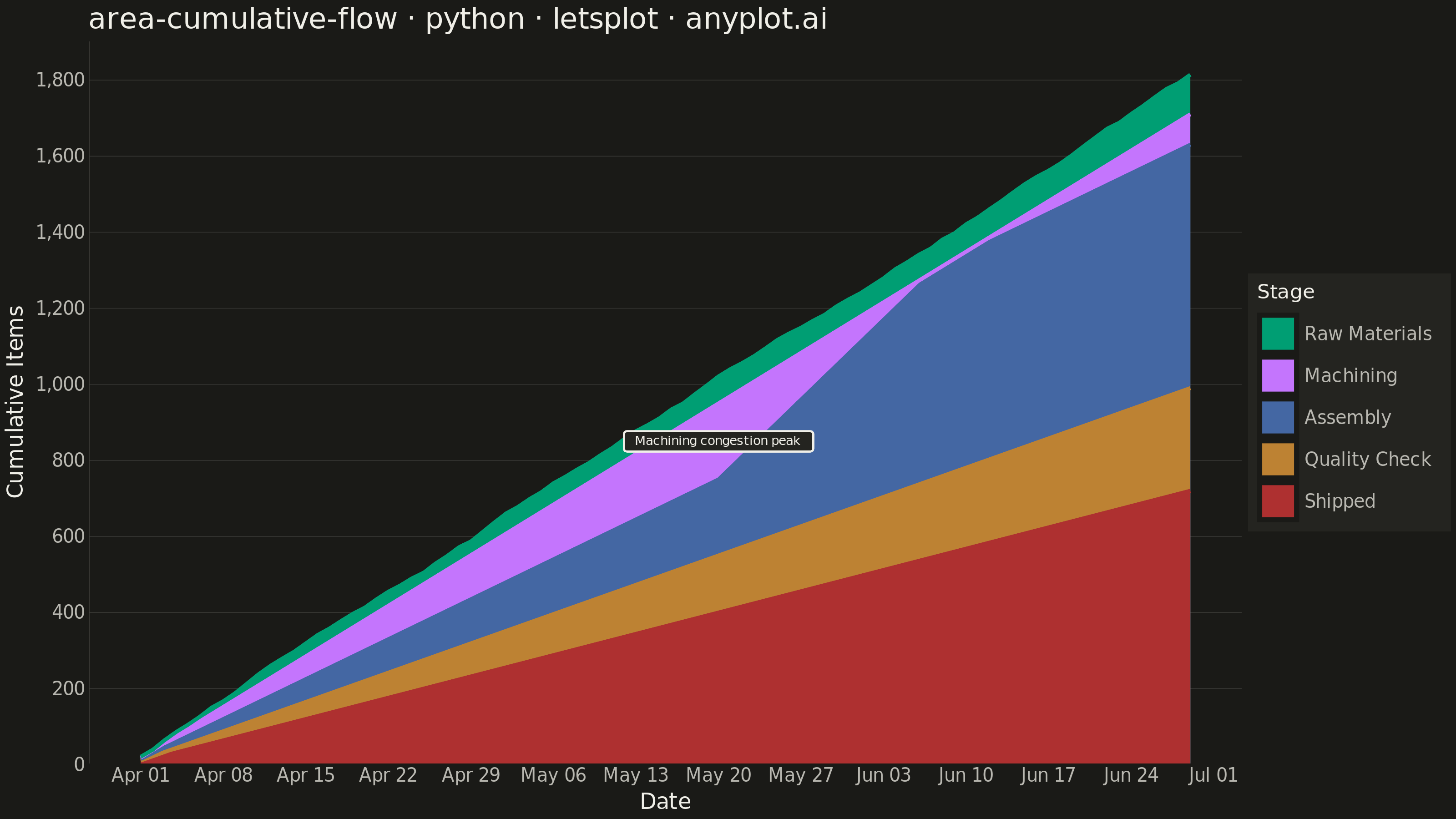
A cumulative flow diagram (CFD) displays the cumulative count of items in each workflow stage as stacked areas over time. Each band represents a stage (e.g., Backlog, In Progress, Done), and the vertical distance between two adjacent band boundaries shows the number of items currently in that stage (work-in-progress). This is a key visualization in Lean and Agile project management for identifying bottlenecks, monitoring throughput, and assessing flow efficiency across a delivery pipeline.
""" anyplot.ai
area-cumulative-flow: Cumulative Flow Diagram for Workflow Analytics
Library: letsplot 4.11.0 | Python 3.13.15
Quality: 94/100 | Created: 2026-08-18
"""

import os

import numpy as np
import pandas as pd
from lets_plot import (
    LetsPlot,
    aes,
    element_blank,
    element_line,
    element_rect,
    element_text,
    geom_area,
    geom_label,
    geom_line,
    ggplot,
    ggsave,
    ggsize,
    ggtitle,
    labs,
    scale_color_manual,
    scale_fill_manual,
    scale_x_datetime,
    theme,
    theme_minimal,
)


LetsPlot.setup_html()

# Theme tokens (see prompts/default-style-guide.md "Background" + "Theme-adaptive Chrome")
THEME = os.getenv("ANYPLOT_THEME", "light")
PAGE_BG = "#FAF8F1" if THEME == "light" else "#1A1A17"
ELEVATED_BG = "#FFFDF6" if THEME == "light" else "#242420"
INK = "#1A1A17" if THEME == "light" else "#F0EFE8"
INK_SOFT = "#4A4A44" if THEME == "light" else "#B8B7B0"
RULE = "rgba(26,26,23,0.15)" if THEME == "light" else "rgba(240,239,232,0.15)"

# Imprint palette (categorical, canonical order) — position 1 always #009E73
IMPRINT_PALETTE = ["#009E73", "#C475FD", "#4467A3", "#BD8233", "#AE3030"]

# Data — a production line's stage-by-stage cumulative item counts (manufacturing CFD)
np.random.seed(42)
n_days = 90
dates = pd.date_range("2024-04-01", periods=n_days, freq="D")
stages = ["Raw Materials", "Machining", "Assembly", "Quality Check", "Shipped"]
base_capacity = [None, 19, 15, 11, 8]  # daily throughput ceiling per downstream stage

daily_intake = np.random.randint(15, 26, size=n_days)
cumulative = np.zeros((len(stages), n_days))
cumulative[0] = np.cumsum(daily_intake)

# Assembly gets a temporary weekend-shift surge (days 50-70) that lifts its
# capacity above Machining's steady output, letting it drain the queue of
# Machining-finished items faster than Machining refills it -- the visible
# Machining band (between the Assembly and Machining curves) narrows during
# that window before widening again once the surge ends, covering both the
# widening- and narrowing-band behaviors named in the spec.
capacity_schedules = []
for stage_idx, cap in enumerate(base_capacity):
    if cap is None:
        capacity_schedules.append(None)
        continue
    schedule = np.full(n_days, cap, dtype=float)
    if stages[stage_idx] == "Assembly":
        schedule[50:70] = 30
    capacity_schedules.append(schedule)

for stage_idx in range(1, len(stages)):
    upstream = cumulative[stage_idx - 1]
    capacity = capacity_schedules[stage_idx]
    processed = 0.0
    for day in range(n_days):
        throughput = min(upstream[day] - processed, capacity[day])
        processed += throughput
        cumulative[stage_idx, day] = processed

# Locate the widest Machining-band moment (pre-surge congestion peak) to call
# out the bottleneck directly rather than leaving it for the viewer to spot.
machining_band_width = cumulative[1] - cumulative[2]
peak_day = int(np.argmax(machining_band_width))
peak_label = pd.DataFrame(
    {
        "date": [dates[peak_day]],
        "count": [(cumulative[1, peak_day] + cumulative[2, peak_day]) / 2],
        "label": ["Machining congestion peak"],
    }
)

# geom_area(position='identity') stacks layers by *factor level* order: the first
# level renders in front, the last level renders behind. The smallest (latest-stage)
# curve must be the first level so it sits in front, and the largest (earliest-stage)
# curve must be the last level so it sits behind and shows through as the top band.
z_order = list(reversed(stages))

flow_df = pd.DataFrame(
    {
        "date": np.tile(dates, len(stages)),
        "stage": pd.Categorical(np.repeat(stages, n_days), categories=z_order, ordered=True),
        "count": cumulative.flatten(),
    }
)

# Plot — see default-style-guide.md "Visual Sizing Defaults" for the canvas + sizing values
plot = (
    ggplot(flow_df, aes(x="date", y="count", fill="stage"))
    + geom_area(position="identity", color=PAGE_BG, size=0.6)
    + geom_line(aes(color="stage"), position="identity", size=0.9, show_legend=False)
    + geom_label(
        aes(x="date", y="count", label="label"),
        data=peak_label,
        inherit_aes=False,
        color=INK,
        fill=ELEVATED_BG,
        size=3.5,
        label_padding=0.3,
    )
    + scale_fill_manual(values=IMPRINT_PALETTE, breaks=stages, name="Stage")
    + scale_color_manual(values=IMPRINT_PALETTE, breaks=stages)
    + scale_x_datetime(format="%b %d")
    + labs(x="Date", y="Cumulative Items")
    + ggtitle("area-cumulative-flow · python · letsplot · anyplot.ai")
    + ggsize(800, 450)
)

# Style — theme-adaptive chrome (see prompts/library/letsplot.md)
plot = (
    plot
    + theme_minimal()
    + theme(
        plot_background=element_rect(fill=PAGE_BG, color=PAGE_BG),
        panel_background=element_rect(fill=PAGE_BG, color=PAGE_BG),
        panel_grid_major_x=element_blank(),
        panel_grid_minor=element_blank(),
        panel_grid_major_y=element_line(color=RULE, size=0.3),
        panel_border=element_blank(),
        axis_title=element_text(color=INK, size=12),
        axis_text=element_text(color=INK_SOFT, size=10),
        axis_line_x=element_line(color=INK_SOFT),
        axis_line_y=element_line(color=INK_SOFT),
        plot_title=element_text(color=INK, size=16),
        legend_background=element_rect(fill=ELEVATED_BG, color=INK_SOFT),
        legend_text=element_text(color=INK_SOFT, size=10),
        legend_title=element_text(color=INK, size=11),
        legend_position="right",
    )
)

# Save
ggsave(plot, f"plot-{THEME}.png", path=".", scale=4)
ggsave(plot, f"plot-{THEME}.html", path=".")
Runnable source as JSON, for any HTTP client: https://api.anyplot.ai/specs/area-cumulative-flow/letsplot/code. Any spec id and library id listed in llms-full.txt fit the same URL shape; every URL below is complete and callable.
{
  "spec_id": "area-cumulative-flow",
  "language": "python",
  "library": "letsplot",
  "page": "https://anyplot.ai/area-cumulative-flow/python/letsplot",
  "hub": "https://anyplot.ai/area-cumulative-flow",
  "code_json": "https://api.anyplot.ai/specs/area-cumulative-flow/letsplot/code",
  "spec_json": "https://api.anyplot.ai/specs/area-cumulative-flow",
  "render_light_png": "https://storage.googleapis.com/anyplot-images/plots/area-cumulative-flow/python/letsplot/plot-light.png",
  "render_dark_png": "https://storage.googleapis.com/anyplot-images/plots/area-cumulative-flow/python/letsplot/plot-dark.png",
  "interactive_light_html": "https://storage.googleapis.com/anyplot-images/plots/area-cumulative-flow/python/letsplot/plot-light.html",
  "interactive_dark_html": "https://storage.googleapis.com/anyplot-images/plots/area-cumulative-flow/python/letsplot/plot-dark.html",
  "quality_score": 94.0,
  "license": "MIT",
  "guide": "https://anyplot.ai/llms.txt"
}
Part of Cumulative Flow Diagram for Workflow Analytics on anyplot.ai.