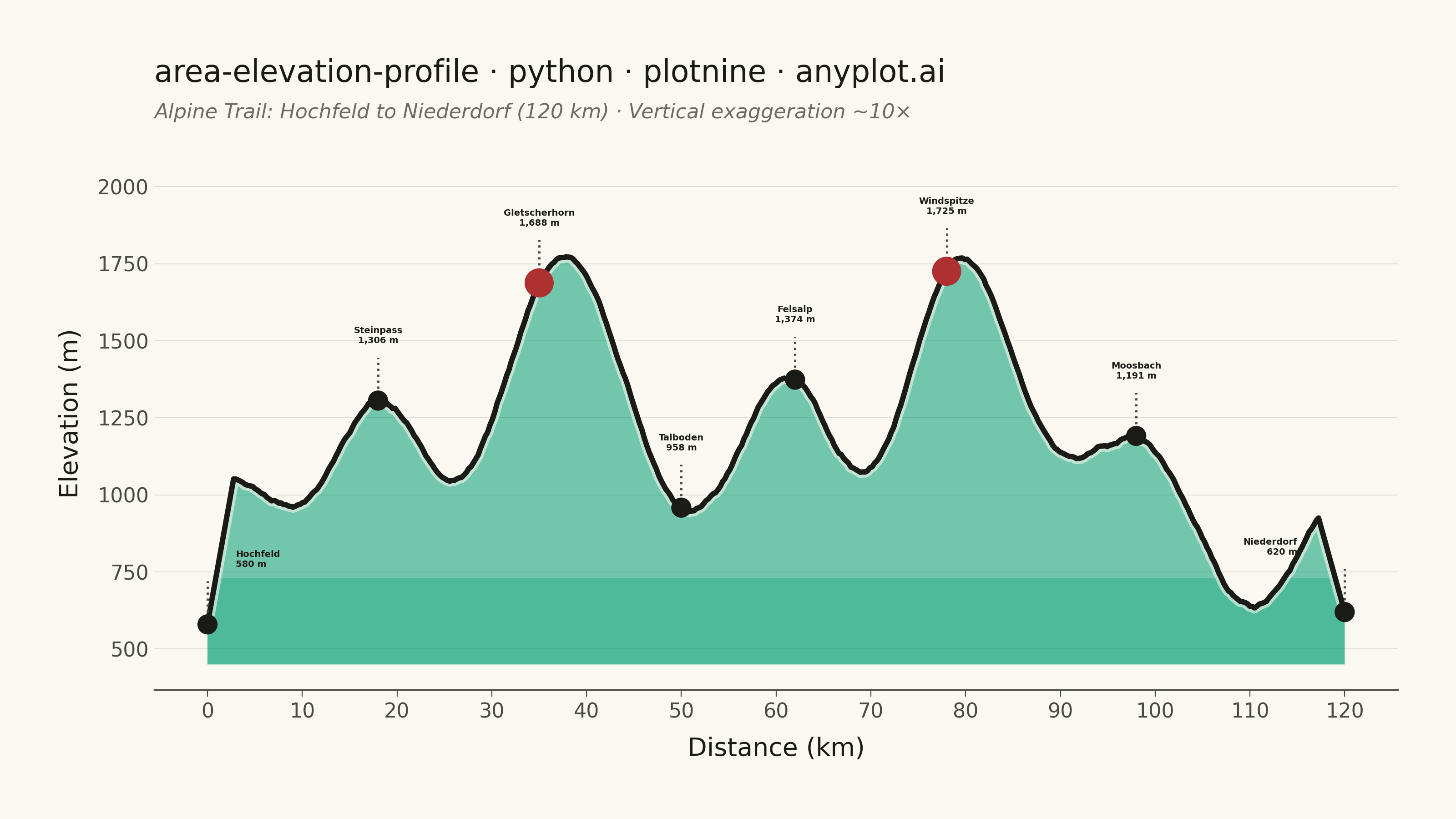
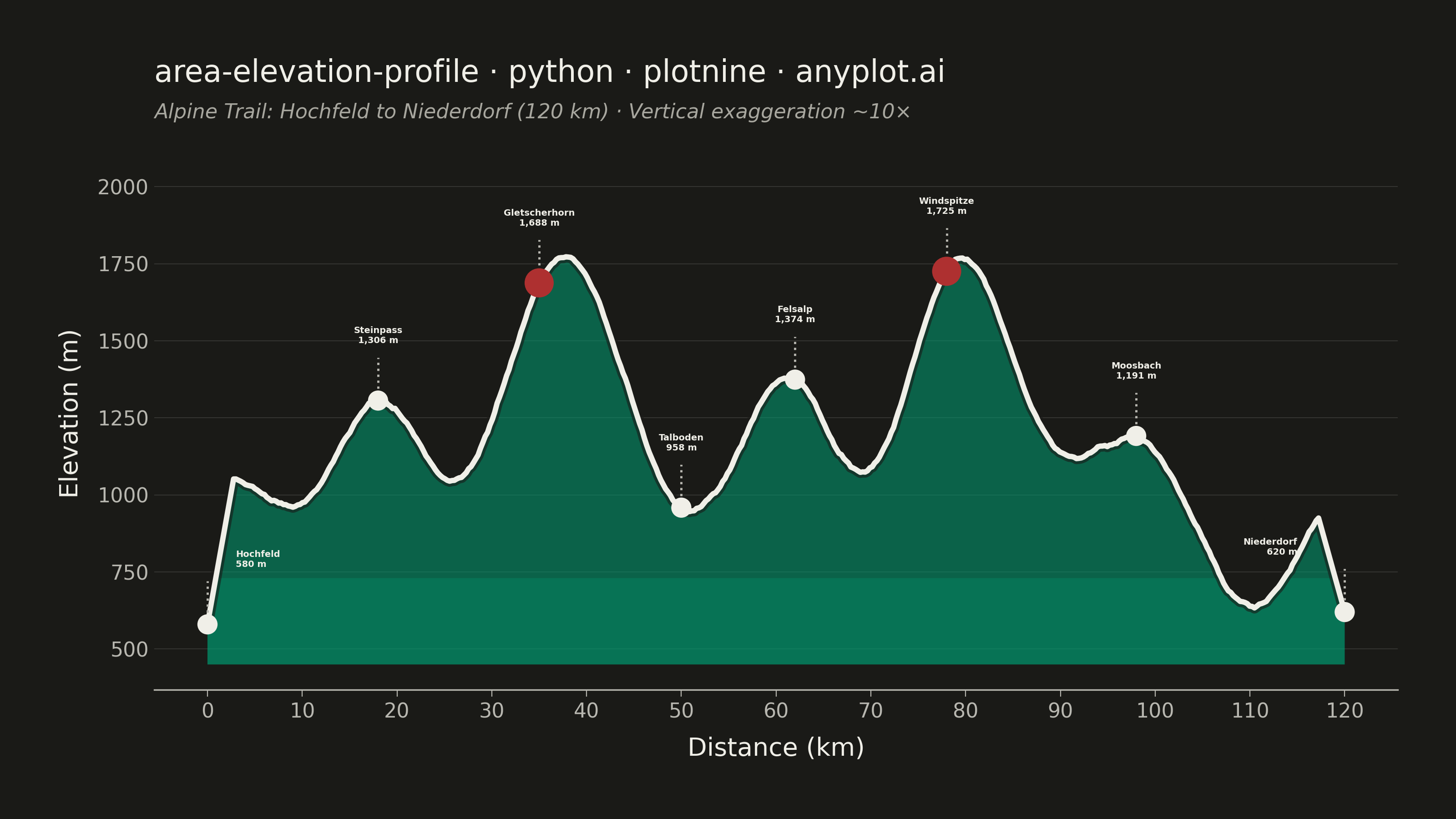
A cross-sectional line plot showing ground elevation along a path or transect line, with the area below the profile filled to create a terrain silhouette. Distance along the transect is plotted on the x-axis and elevation on the y-axis. This visualization is widely used in hiking and cycling route planning, civil engineering corridor design, and geomorphology to convey terrain shape and difficulty at a glance.
""" anyplot.ai
area-elevation-profile: Terrain Elevation Profile Along Transect
Library: plotnine 0.15.5 | Python 3.13.13
Quality: 91/100 | Updated: 2026-06-10
"""

import os

import numpy as np
import pandas as pd
from plotnine import (
    aes,
    coord_cartesian,
    element_blank,
    element_line,
    element_rect,
    element_text,
    geom_line,
    geom_point,
    geom_ribbon,
    geom_segment,
    geom_text,
    ggplot,
    labs,
    scale_x_continuous,
    scale_y_continuous,
    theme,
    theme_minimal,
)


# Theme tokens
THEME = os.getenv("ANYPLOT_THEME", "light")
PAGE_BG = "#FAF8F1" if THEME == "light" else "#1A1A17"
ELEVATED_BG = "#FFFDF6" if THEME == "light" else "#242420"
INK = "#1A1A17" if THEME == "light" else "#F0EFE8"
INK_SOFT = "#4A4A44" if THEME == "light" else "#B8B7B0"
INK_MUTED = "#6B6A63" if THEME == "light" else "#A8A79F"
BRAND = "#009E73"  # Imprint palette position 1 — terrain fill
SUMMIT_COLOR = "#AE3030"  # Imprint palette position 5 — high-peak emphasis

# Data — Alpine hiking trail elevation profile (~120 km), fictional location names
np.random.seed(42)
n_points = 480
distance = np.linspace(0, 120, n_points)

# Terrain with controlled Gaussian peaks at landmark locations
elevation = np.full(n_points, 800.0)
elevation += 500 * np.exp(-((distance - 18) ** 2) / 50)
elevation += 900 * np.exp(-((distance - 35) ** 2) / 80)
elevation += 650 * np.exp(-((distance - 62) ** 2) / 60)
elevation += 750 * np.exp(-((distance - 78) ** 2) / 70)
elevation += 400 * np.exp(-((distance - 98) ** 2) / 90)
elevation += 200 * np.sin(distance * np.pi / 20 + 0.8)
elevation += 100 * np.sin(distance * np.pi / 10 + 1.5)
elevation += np.random.normal(0, 15, n_points)
elevation = pd.Series(elevation).rolling(window=8, center=True, min_periods=1).mean().values.copy()
elevation[:12] = np.linspace(580, elevation[12], 12)
elevation[-12:] = np.linspace(elevation[-12], 620, 12)

y_min = 450
y_max = int(np.ceil(elevation.max() / 100) * 100) + 280
shadow_top = y_min + 280  # narrow base shadow band for elevation-depth effect

df = pd.DataFrame(
    {"distance": distance, "elevation": elevation, "y_min": y_min, "shadow_level": np.minimum(elevation, shadow_top)}
)

# Landmarks with fictional Alpine names to avoid real-world elevation mismatches
landmarks = pd.DataFrame(
    {
        "name": [
            "Hochfeld",
            "Steinpass",
            "Gletscherhorn",
            "Talboden",
            "Felsalp",
            "Windspitze",
            "Moosbach",
            "Niederdorf",
        ],
        "distance": [0, 18, 35, 50, 62, 78, 98, 120],
    }
)
landmarks["elevation"] = landmarks["distance"].apply(lambda d: elevation[np.argmin(np.abs(distance - d))])
landmarks["label_y"] = landmarks["elevation"] + 180
landmarks["label"] = landmarks.apply(lambda r: f"{r['name']}\n{int(r['elevation']):,} m", axis=1)
landmarks["ha"] = "center"
landmarks.loc[landmarks["distance"] < 5, "ha"] = "left"
landmarks.loc[landmarks["distance"] > 115, "ha"] = "right"
landmarks["seg_top"] = landmarks["elevation"] + 140

# Mark top-2 highest landmarks as summits for distinct visual emphasis
summit_threshold = landmarks["elevation"].nlargest(2).min()
landmarks["is_summit"] = landmarks["elevation"] >= summit_threshold
summits = landmarks[landmarks["is_summit"]]
valleys = landmarks[~landmarks["is_summit"]]

# Title length-scaled fontsize (67-char baseline = 12pt)
title = "area-elevation-profile · python · plotnine · anyplot.ai"
n = len(title)
ratio = 67 / n if n > 67 else 1.0
title_fontsize = max(8, round(12 * ratio))

# Plot
plot = (
    ggplot(df, aes(x="distance", y="elevation"))
    # Two-layer terrain: full fill + base shadow band for elevation depth
    + geom_ribbon(aes(ymin="y_min", ymax="elevation"), fill=BRAND, alpha=0.55)
    + geom_ribbon(aes(ymin="y_min", ymax="shadow_level"), fill=BRAND, alpha=0.30)
    # Profile line with PAGE_BG halo for visual separation from terrain fill
    + geom_line(color=PAGE_BG, size=2.5, alpha=0.6)
    + geom_line(color=INK, size=1.2)
    # Vertical marker lines from landmark point up to label
    + geom_segment(
        aes(x="distance", xend="distance", y="elevation", yend="seg_top"),
        data=landmarks,
        color=INK_SOFT,
        linetype="dotted",
        size=0.5,
    )
    # Valley markers
    + geom_point(aes(x="distance", y="elevation"), data=valleys, size=3.5, color=INK)
    # Summit markers — larger and accent-colored for high-point drama
    + geom_point(aes(x="distance", y="elevation"), data=summits, size=5.5, color=SUMMIT_COLOR)
    # Left-aligned edge labels (nudged inward)
    + geom_text(
        aes(x="distance", y="label_y", label="label"),
        data=landmarks[landmarks["ha"] == "left"],
        size=3.5,
        color=INK,
        ha="left",
        va="bottom",
        fontweight="bold",
        nudge_x=3,
    )
    # Center-aligned labels
    + geom_text(
        aes(x="distance", y="label_y", label="label"),
        data=landmarks[landmarks["ha"] == "center"],
        size=3.5,
        color=INK,
        ha="center",
        va="bottom",
        fontweight="bold",
    )
    # Right-aligned edge labels (nudged inward)
    + geom_text(
        aes(x="distance", y="label_y", label="label"),
        data=landmarks[landmarks["ha"] == "right"],
        size=3.5,
        color=INK,
        ha="right",
        va="bottom",
        fontweight="bold",
        nudge_x=-5,
    )
    + labs(
        x="Distance (km)",
        y="Elevation (m)",
        title=title,
        subtitle="Alpine Trail: Hochfeld to Niederdorf (120 km) · Vertical exaggeration ~10×",
    )
    + scale_x_continuous(breaks=range(0, 130, 10), expand=(0.03, 2))
    + scale_y_continuous(breaks=range(500, 2200, 250))
    + coord_cartesian(ylim=(y_min, y_max))
    + theme_minimal()
    + theme(
        figure_size=(8, 4.5),
        text=element_text(size=7, color=INK),
        axis_title=element_text(size=10, color=INK),
        axis_text=element_text(size=8, color=INK_SOFT),
        plot_title=element_text(size=title_fontsize, color=INK),
        plot_subtitle=element_text(size=8, color=INK_MUTED, style="italic"),
        legend_text=element_text(size=8, color=INK_SOFT),
        panel_background=element_rect(fill=PAGE_BG, color="none"),
        plot_background=element_rect(fill=PAGE_BG, color="none"),
        panel_grid_major_y=element_line(color=INK, size=0.3, alpha=0.15),
        panel_grid_major_x=element_blank(),
        panel_grid_minor=element_blank(),
        panel_border=element_blank(),
        axis_line_x=element_line(color=INK_SOFT, size=0.6),
        axis_ticks_major_x=element_line(color=INK_SOFT, size=0.4),
        axis_ticks_major_y=element_blank(),
        plot_margin=0.04,
    )
)

# Save
plot.save(f"plot-{THEME}.png", dpi=400, width=8, height=4.5, units="in", verbose=False)
Runnable source as JSON, for any HTTP client: https://api.anyplot.ai/specs/area-elevation-profile/plotnine/code. Any spec id and library id listed in llms-full.txt fit the same URL shape; every URL below is complete and callable.
{
  "spec_id": "area-elevation-profile",
  "language": "python",
  "library": "plotnine",
  "page": "https://anyplot.ai/area-elevation-profile/python/plotnine",
  "hub": "https://anyplot.ai/area-elevation-profile",
  "code_json": "https://api.anyplot.ai/specs/area-elevation-profile/plotnine/code",
  "spec_json": "https://api.anyplot.ai/specs/area-elevation-profile",
  "render_light_png": "https://storage.googleapis.com/anyplot-images/plots/area-elevation-profile/python/plotnine/plot-light.png",
  "render_dark_png": "https://storage.googleapis.com/anyplot-images/plots/area-elevation-profile/python/plotnine/plot-dark.png",
  "quality_score": 91.0,
  "license": "MIT",
  "guide": "https://anyplot.ai/llms.txt"
}
Part of Terrain Elevation Profile Along Transect on anyplot.ai.