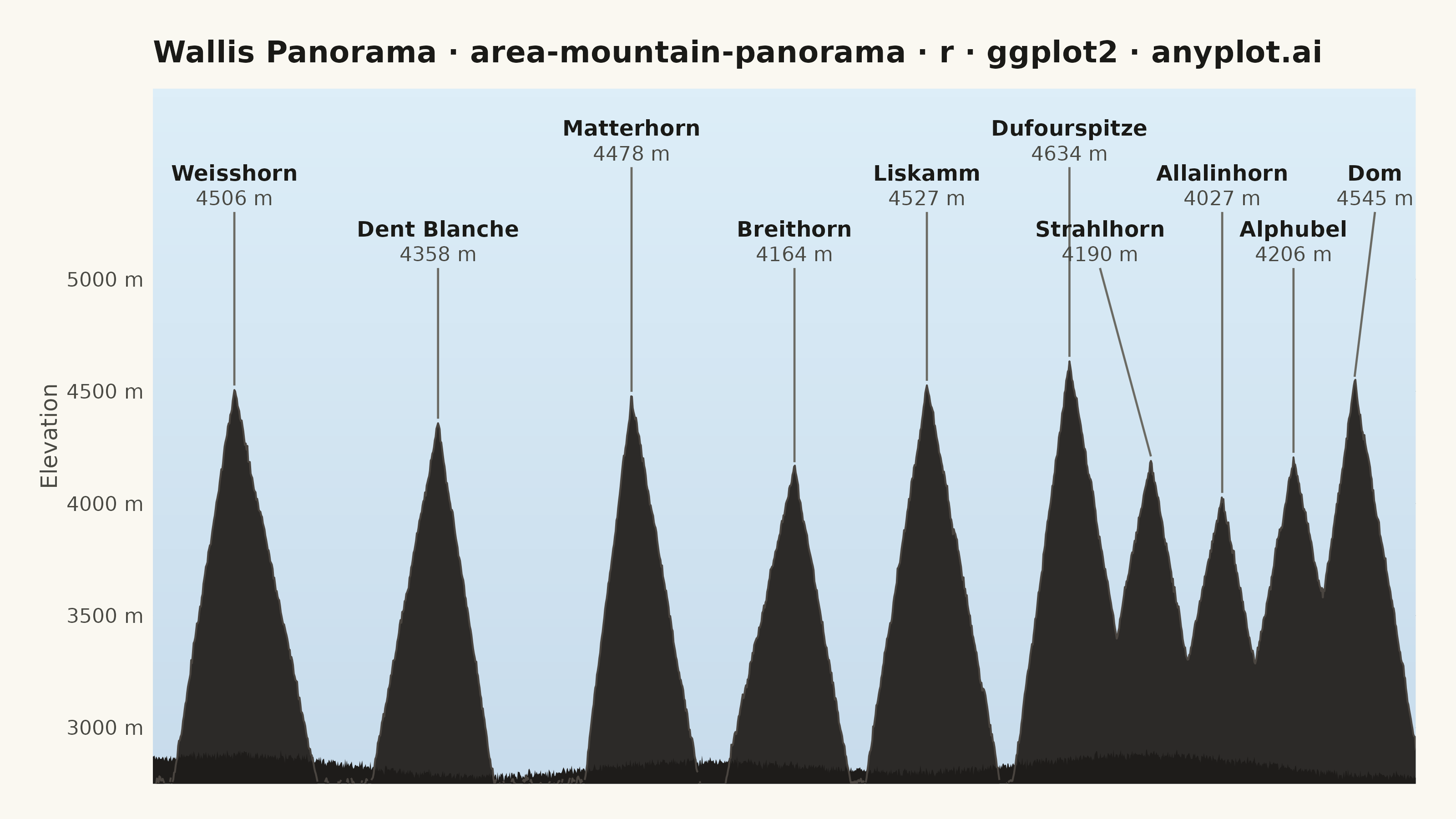
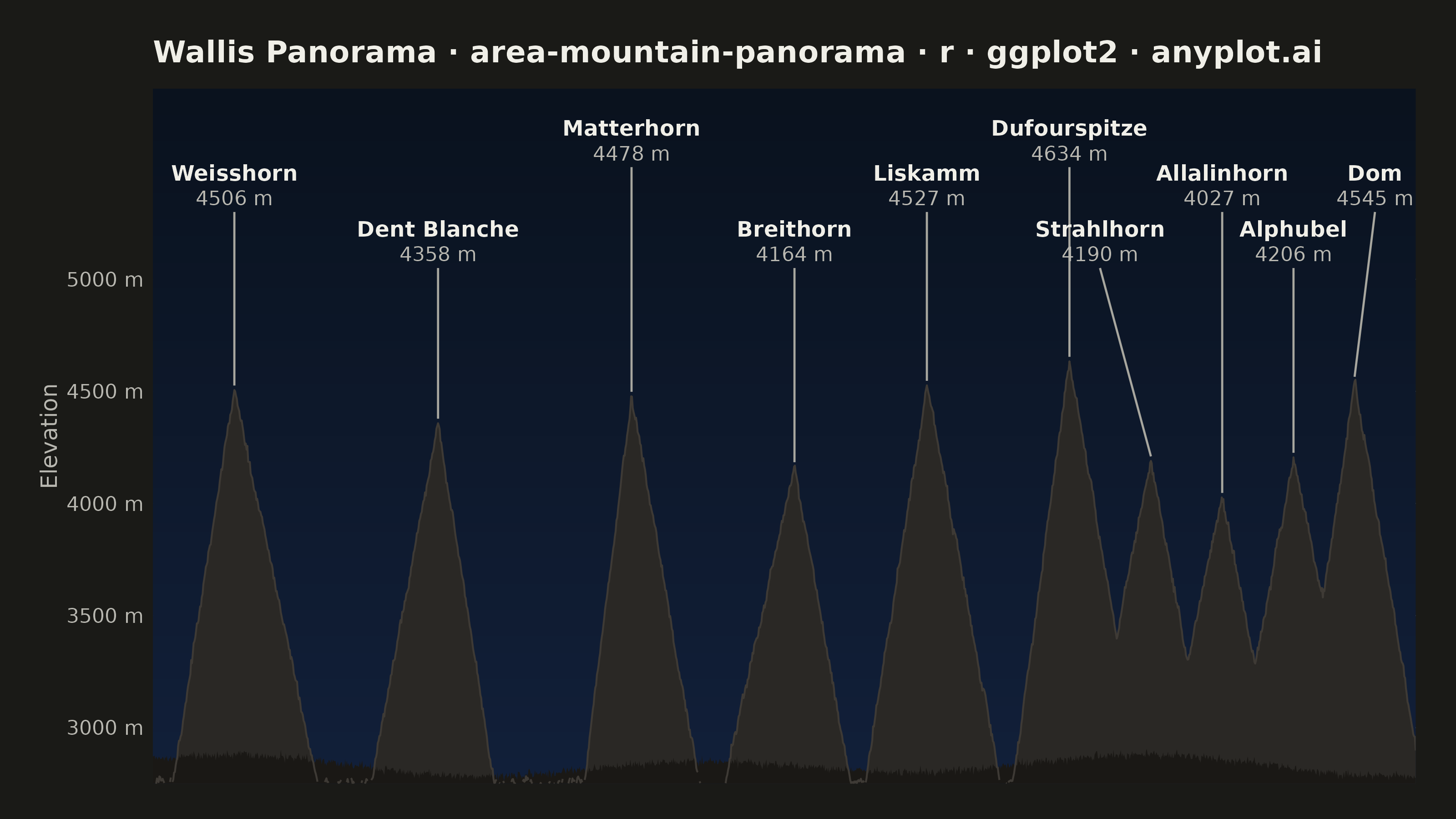
The same plot in 14 other libraries — Python: Altair, Bokeh, lets-plot, Matplotlib, Plotly, plotnine, Pygal, Seaborn; Julia: Makie.jl; JavaScript: Chart.js, D3.js, Apache ECharts, Highcharts, MUI X Charts. Compare all 15 side by side: Mountain Panorama Profile with Labeled Peaks in Python, R, Julia and JavaScript.
A panoramic mountain silhouette chart that renders the horizon as seen from a fixed vantage point, like a photograph of a ridgeline against the sky. A filled area under the skyline curve traces the ridgeline across a horizontal viewing range (in degrees of bearing or horizontal distance), and major summits are annotated with their name and elevation. The skyline is jagged and angular — sharp triangular peaks with steep, often asymmetric flanks meeting at pointed apexes, connected by rugged ridges with cols, sub-peaks and rocky notches — not a sequence of smooth bell-shaped bumps. Unlike an elevation-profile-along-a-trail, this plot is the angular view of the surrounding peaks from a single observer, making it ideal for summit-identification infographics, alpine panoramas, and travel guides.
#' anyplot.ai
#' area-mountain-panorama: Mountain Panorama Profile with Labeled Peaks
#' Library: ggplot2 3.5.1 | R 4.4.1
#' Quality: 89/100 | Created: 2026-06-30

library(ggplot2)
library(ragg)

set.seed(42)

# Theme tokens
THEME       <- Sys.getenv("ANYPLOT_THEME", "light")
PAGE_BG     <- if (THEME == "light") "#FAF8F1" else "#1A1A17"
INK         <- if (THEME == "light") "#1A1A17" else "#F0EFE8"
INK_SOFT    <- if (THEME == "light") "#4A4A44" else "#B8B7B0"
INK_MUTED   <- if (THEME == "light") "#6B6A63" else "#A8A79F"

# Panorama-specific colors (atmospheric tones, not categorical palette)
SKY_BOTTOM    <- if (THEME == "light") "#C8DCEC" else "#12203A"
SKY_TOP       <- if (THEME == "light") "#DDEEF8" else "#0A121E"
MOUNTAIN_FILL <- if (THEME == "light") "#2C2A28" else "#2A2825"
MOUNTAIN_FG   <- if (THEME == "light") "#1E1C1A" else "#1A1815"
RIDGE_COLOR   <- if (THEME == "light") "#4A4540" else "#3E3A35"

# Peak data: Wallis panorama — 10 summits in a west-to-east sweep
peaks_df <- data.frame(
  name      = c("Weisshorn", "Dent Blanche", "Matterhorn", "Breithorn",
                "Liskamm", "Dufourspitze", "Strahlhorn", "Allalinhorn",
                "Alphubel", "Dom"),
  angle_deg = c(  8,  28,  47,  63,  76,  90,  98, 105, 112, 118),
  elev_m    = c(4506, 4358, 4478, 4164, 4527, 4634, 4190, 4027, 4206, 4545),
  stringsAsFactors = FALSE
)

# Label stagger heights — SPECIAL for focal peaks, alternating HIGH/LOW for rest
peaks_df$label_y <- c(
  5300,  # Weisshorn     HIGH
  5050,  # Dent Blanche  LOW
  5500,  # Matterhorn    SPECIAL (focal)
  5050,  # Breithorn     LOW
  5300,  # Liskamm       HIGH
  5500,  # Dufourspitze  SPECIAL (highest)
  5050,  # Strahlhorn    LOW
  5300,  # Allalinhorn   HIGH
  5050,  # Alphubel      LOW
  5300   # Dom           HIGH
)

# Horizontal label positions — spread dense right cluster (Strahlhorn–Dom in 20° span)
peaks_df$label_x <- c(
   8,   # Weisshorn
  28,   # Dent Blanche
  47,   # Matterhorn
  63,   # Breithorn
  76,   # Liskamm
  90,   # Dufourspitze
  93,   # Strahlhorn (nudged left from 98°)
 105,   # Allalinhorn
 112,   # Alphubel
 120    # Dom (nudged right from 118°, 4° from right edge)
)

# Derived label positions
peaks_df$seg_y1 <- peaks_df$label_y
peaks_df$elev_y <- peaks_df$label_y + 30
peaks_df$name_y <- peaks_df$label_y + 30 + 80 + 30

# Skyline: sum of tent functions (asymmetric flanks) + smoothed noise
BASE_ELEV <- 2750
angles    <- seq(0, 124, by = 0.08)
n_pts     <- length(angles)

slp_left  <- c(290, 245, 370, 205, 295, 340, 230, 215, 245, 315)
slp_right <- c(215, 290, 260, 255, 245, 265, 250, 230, 220, 270)

skyline <- rep(BASE_ELEV, n_pts)
for (i in seq_len(nrow(peaks_df))) {
  pa   <- peaks_df$angle_deg[i]
  pe   <- peaks_df$elev_m[i]
  tent <- ifelse(angles <= pa,
                 pe - slp_left[i]  * (pa - angles),
                 pe - slp_right[i] * (angles - pa))
  skyline <- pmax(skyline, pmax(tent, BASE_ELEV))
}

# Ridge jaggedness: smoothed noise + micro-roughness
noise_sm <- as.numeric(stats::filter(rnorm(n_pts, 0, 28), rep(1 / 7, 7), sides = 2))
noise_sm[is.na(noise_sm)] <- 0
skyline <- skyline + noise_sm + rnorm(n_pts, 0, 9)

# Re-anchor named summits to exact elevations
for (i in seq_len(nrow(peaks_df))) {
  skyline[which.min(abs(angles - peaks_df$angle_deg[i]))] <- peaks_df$elev_m[i]
}

panorama_df <- data.frame(angle = angles, elev = skyline)

# Foreground ridge: closer terrain adding visual depth
fg_ridge <- BASE_ELEV + 80 +
  35 * sin(angles * 0.14 + 0.4) +
  18 * cos(angles * 0.07) +
  rnorm(n_pts, 0, 10)
fg_df <- data.frame(angle = angles, ridge = fg_ridge)

# Sky gradient raster — top row (ymax) = SKY_TOP, bottom row (ymin) = SKY_BOTTOM
n_sky    <- 80
sky_grad <- colorRampPalette(c(SKY_TOP, SKY_BOTTOM))(n_sky)
sky_mat  <- matrix(sky_grad, nrow = n_sky, ncol = 1)

# Title — 67 chars → ratio = 1.0 → title_size = 12
title_str  <- "Wallis Panorama · area-mountain-panorama · r · ggplot2 · anyplot.ai"
title_n    <- nchar(title_str)
title_size <- max(8, round(12 * 67 / title_n))

p <- ggplot() +
  # Sky gradient background (annotation_raster: row 1 = ymax = top)
  annotation_raster(
    raster      = sky_mat,
    xmin        = 0,
    xmax        = 124,
    ymin        = BASE_ELEV,
    ymax        = 5850,
    interpolate = TRUE
  ) +
  # Main mountain silhouette
  geom_ribbon(
    data  = panorama_df,
    aes(x = angle, ymin = BASE_ELEV, ymax = elev),
    fill  = MOUNTAIN_FILL,
    color = NA
  ) +
  # Foreground ridge (depth layer)
  geom_ribbon(
    data  = fg_df,
    aes(x = angle, ymin = BASE_ELEV, ymax = ridge),
    fill  = MOUNTAIN_FG,
    color = NA
  ) +
  # Ridgeline edge
  geom_line(
    data      = panorama_df,
    aes(x = angle, y = elev),
    color     = RIDGE_COLOR,
    linewidth = 0.35
  ) +
  # Leader lines: summit tip → label base (angled to spread-label positions)
  geom_segment(
    data = peaks_df,
    aes(x = angle_deg, xend = label_x, y = elev_m + 20, yend = seg_y1),
    color     = INK_MUTED,
    linewidth = 0.4
  ) +
  # Elevation labels
  geom_text(
    data     = peaks_df,
    aes(x = label_x, y = elev_y, label = paste0(elev_m, " m")),
    color    = INK_SOFT,
    size     = 2.8,
    hjust    = 0.5,
    vjust    = 0
  ) +
  # Peak names (bold, above elevation)
  geom_text(
    data     = peaks_df,
    aes(x = label_x, y = name_y, label = name),
    color    = INK,
    size     = 3.0,
    hjust    = 0.5,
    vjust    = 0,
    fontface = "bold"
  ) +
  scale_x_continuous(limits = c(0, 124), expand = expansion(0)) +
  scale_y_continuous(
    limits = c(BASE_ELEV, 5850),
    breaks = c(3000, 3500, 4000, 4500, 5000),
    labels = function(x) paste0(x, " m"),
    expand = expansion(0)
  ) +
  labs(title = title_str, x = NULL, y = "Elevation") +
  theme_minimal(base_size = 8) +
  theme(
    plot.background    = element_rect(fill = PAGE_BG, color = PAGE_BG),
    panel.background   = element_rect(fill = NA,      color = NA),
    panel.grid.major.y = element_line(color = INK_MUTED, linewidth = 0.15,
                                      linetype = "dashed"),
    panel.grid.major.x = element_blank(),
    panel.grid.minor   = element_blank(),
    panel.border       = element_blank(),
    axis.title.x       = element_blank(),
    axis.text.x        = element_blank(),
    axis.ticks.x       = element_blank(),
    axis.title.y       = element_text(color = INK_SOFT, size = 9),
    axis.text.y        = element_text(color = INK_SOFT, size = 8),
    axis.ticks.y       = element_blank(),
    plot.title         = element_text(color = INK, size = title_size,
                                      face = "bold",
                                      margin = margin(b = 8)),
    plot.margin        = margin(16, 16, 12, 16, unit = "pt")
  )

ggsave(
  filename = sprintf("plot-%s.png", THEME),
  plot     = p,
  device   = ragg::agg_png,
  width    = 8,
  height   = 4.5,
  units    = "in",
  dpi      = 400
)
Runnable source as JSON, for any HTTP client: https://api.anyplot.ai/specs/area-mountain-panorama/ggplot2/code. Any spec id and library id listed in llms-full.txt fit the same URL shape; every URL below is complete and callable.
{
  "spec_id": "area-mountain-panorama",
  "language": "r",
  "library": "ggplot2",
  "page": "https://anyplot.ai/area-mountain-panorama/r/ggplot2",
  "hub": "https://anyplot.ai/area-mountain-panorama",
  "code_json": "https://api.anyplot.ai/specs/area-mountain-panorama/ggplot2/code",
  "spec_json": "https://api.anyplot.ai/specs/area-mountain-panorama",
  "render_light_png": "https://storage.googleapis.com/anyplot-images/plots/area-mountain-panorama/r/ggplot2/plot-light.png",
  "render_dark_png": "https://storage.googleapis.com/anyplot-images/plots/area-mountain-panorama/r/ggplot2/plot-dark.png",
  "quality_score": 89.0,
  "license": "MIT",
  "guide": "https://anyplot.ai/llms.txt"
}
Part of Mountain Panorama Profile with Labeled Peaks on anyplot.ai.