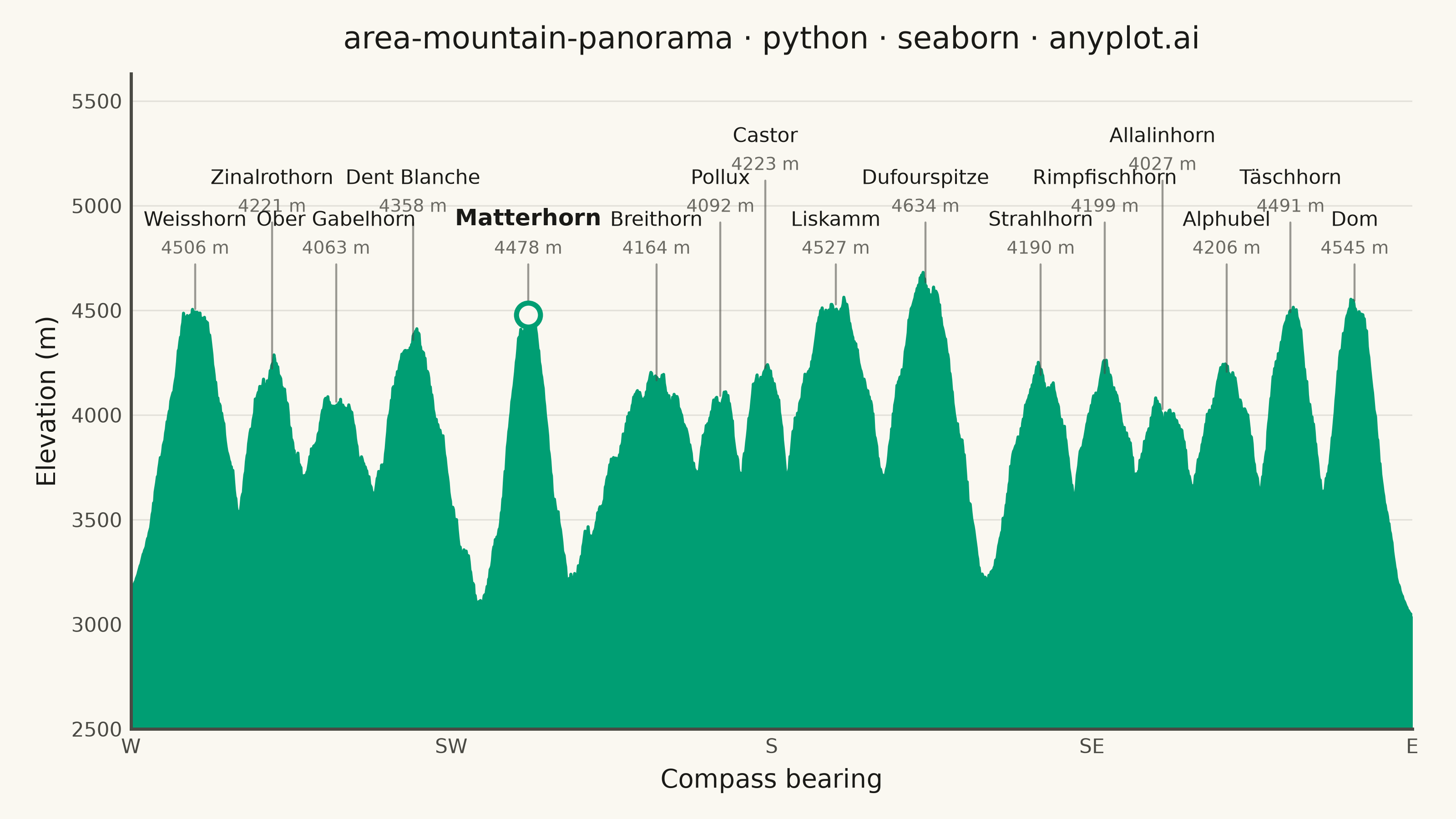
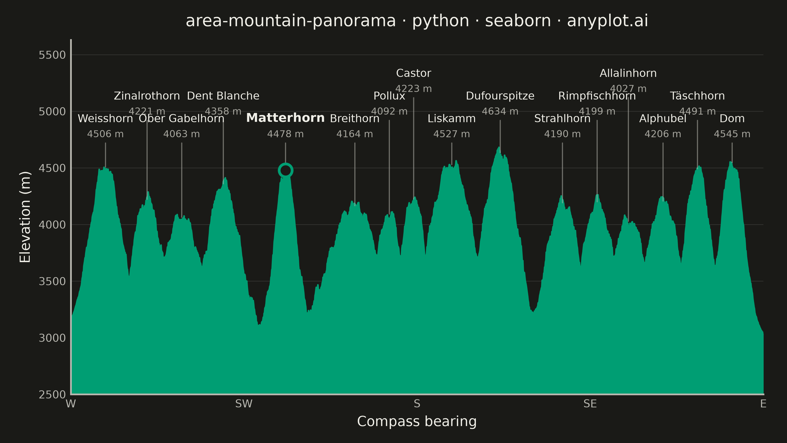
A panoramic mountain silhouette chart that renders the horizon as seen from a fixed vantage point, like a photograph of a ridgeline against the sky. A filled area under the skyline curve traces the ridgeline across a horizontal viewing range (in degrees of bearing or horizontal distance), and major summits are annotated with their name and elevation. The skyline is jagged and angular — sharp triangular peaks with steep, often asymmetric flanks meeting at pointed apexes, connected by rugged ridges with cols, sub-peaks and rocky notches — not a sequence of smooth bell-shaped bumps. Unlike an elevation-profile-along-a-trail, this plot is the angular view of the surrounding peaks from a single observer, making it ideal for summit-identification infographics, alpine panoramas, and travel guides.
""" anyplot.ai
area-mountain-panorama: Mountain Panorama Profile with Labeled Peaks
Library: seaborn 0.13.2 | Python 3.13.14
Quality: 87/100 | Updated: 2026-06-30
"""

import os

import matplotlib.pyplot as plt
import numpy as np
import pandas as pd
import seaborn as sns
from matplotlib.colors import LinearSegmentedColormap


# Theme tokens
THEME = os.getenv("ANYPLOT_THEME", "light")
PAGE_BG = "#FAF8F1" if THEME == "light" else "#1A1A17"
ELEVATED_BG = "#FFFDF6" if THEME == "light" else "#242420"
INK = "#1A1A17" if THEME == "light" else "#F0EFE8"
INK_SOFT = "#4A4A44" if THEME == "light" else "#B8B7B0"
INK_MUTED = "#6B6A63" if THEME == "light" else "#A8A79F"
BRAND = "#009E73"

sns.set_theme(
    style="ticks",
    rc={
        "figure.facecolor": PAGE_BG,
        "axes.facecolor": PAGE_BG,
        "axes.edgecolor": INK_SOFT,
        "axes.labelcolor": INK,
        "text.color": INK,
        "xtick.color": INK_SOFT,
        "ytick.color": INK_SOFT,
        "grid.color": INK,
        "grid.alpha": 0.10,
        "legend.facecolor": ELEVATED_BG,
        "legend.edgecolor": INK_SOFT,
    },
)

# Data — Wallis (Valais, Switzerland) panorama from Gornergrat, west → east sweep.
# left_slope / right_slope: angular half-width (degrees) per unit drop on each flank.
# Smaller = steeper spike. Asymmetry per peak gives varied alpine silhouette.
# Matterhorn gets very narrow slopes to create the iconic sharp spike even though it is
# not the tallest peak — its narrow tent makes it visually pierce the ridgeline.
peaks = pd.DataFrame(
    [
        {"name": "Weisshorn", "angle_deg": 10.0, "elevation_m": 4506, "left_slope": 5.0, "right_slope": 7.0},
        {"name": "Zinalrothorn", "angle_deg": 22.0, "elevation_m": 4221, "left_slope": 4.0, "right_slope": 5.5},
        {"name": "Ober Gabelhorn", "angle_deg": 32.0, "elevation_m": 4063, "left_slope": 6.5, "right_slope": 4.5},
        {"name": "Dent Blanche", "angle_deg": 44.0, "elevation_m": 4358, "left_slope": 5.5, "right_slope": 7.0},
        {"name": "Matterhorn", "angle_deg": 62.0, "elevation_m": 4478, "left_slope": 2.8, "right_slope": 2.0},
        {"name": "Breithorn", "angle_deg": 82.0, "elevation_m": 4164, "left_slope": 8.5, "right_slope": 6.5},
        {"name": "Pollux", "angle_deg": 92.0, "elevation_m": 4092, "left_slope": 3.5, "right_slope": 4.5},
        {"name": "Castor", "angle_deg": 99.0, "elevation_m": 4223, "left_slope": 3.5, "right_slope": 3.0},
        {"name": "Liskamm", "angle_deg": 110.0, "elevation_m": 4527, "left_slope": 8.0, "right_slope": 5.5},
        {"name": "Dufourspitze", "angle_deg": 124.0, "elevation_m": 4634, "left_slope": 6.5, "right_slope": 5.0},
        {"name": "Strahlhorn", "angle_deg": 142.0, "elevation_m": 4190, "left_slope": 5.5, "right_slope": 6.0},
        {"name": "Rimpfischhorn", "angle_deg": 152.0, "elevation_m": 4199, "left_slope": 4.0, "right_slope": 5.5},
        {"name": "Allalinhorn", "angle_deg": 161.0, "elevation_m": 4027, "left_slope": 5.5, "right_slope": 4.0},
        {"name": "Alphubel", "angle_deg": 171.0, "elevation_m": 4206, "left_slope": 6.0, "right_slope": 4.5},
        {"name": "Täschhorn", "angle_deg": 181.0, "elevation_m": 4491, "left_slope": 4.5, "right_slope": 3.5},
        {"name": "Dom", "angle_deg": 191.0, "elevation_m": 4545, "left_slope": 4.0, "right_slope": 5.5},
    ]
)

# Build skyline as upper envelope of piecewise-linear tent functions over undulating valley floor.
# Tent formula: bump = h * max(0, 1 - left_dist - right_dist)
# Exactly one of {left_dist, right_dist} is nonzero at each sample — giving sharp apexes.
# Saddles between peaks dip to the valley floor because tent is zero beyond slope*1 deg.
np.random.seed(42)
sample_angles = np.linspace(-5.0, 205.0, 1800)

valley_floor = 2950 + 90 * np.sin(sample_angles * np.pi / 95.0 + 0.4) + 55 * np.cos(sample_angles * np.pi / 47.0 + 1.1)

ridge = np.copy(valley_floor)
for _, row in peaks.iterrows():
    floor_at_peak = valley_floor[np.argmin(np.abs(sample_angles - row["angle_deg"]))]
    bump_height = row["elevation_m"] - floor_at_peak
    left_dist = np.clip((row["angle_deg"] - sample_angles) / row["left_slope"], 0.0, None)
    right_dist = np.clip((sample_angles - row["angle_deg"]) / row["right_slope"], 0.0, None)
    tent = bump_height * np.maximum(0.0, 1.0 - left_dist - right_dist)
    ridge = np.maximum(ridge, valley_floor + tent)

# Small rocky texture along ridgeline (jagged detail), tapered at panorama edges
texture = (
    20 * np.sin(sample_angles * 1.7 + 0.3)
    + 12 * np.sin(sample_angles * 3.1 + 1.7)
    + np.random.normal(0, 9, size=sample_angles.shape)
)
edge_taper = np.clip((sample_angles - 0) / 6, 0, 1) * np.clip((200 - sample_angles) / 6, 0, 1)
ridge = ridge + texture * edge_taper

skyline = pd.DataFrame({"angle_deg": sample_angles, "elevation_m": ridge})

# Canvas: 3200×1800 px (figsize=(8,4.5) × dpi=400)
fig, ax = plt.subplots(figsize=(8, 4.5), dpi=400, facecolor=PAGE_BG)
ax.set_facecolor(PAGE_BG)

Y_FLOOR = 2500
LABEL_BASE_Y = 4880
LABEL_STAGGER = 200
Y_TOP = LABEL_BASE_Y + 2 * LABEL_STAGGER + 350  # 5630

# Dusk sky gradient above ridgeline — the mountain silhouette (zorder=2) covers below the ridge;
# the gradient is visible in the sky and annotation zones above it.
sky_colors = (
    ["#FDDCB0", "#E8A870", "#A8C8E0"]  # warm amber → golden → soft sky blue
    if THEME == "light"
    else ["#6B2040", "#2A1860", "#0A1428"]  # magenta-purple → indigo → near-black
)
sky_cmap = LinearSegmentedColormap.from_list("sky_dusk", sky_colors)
sky_arr = np.linspace(0, 1, 256).reshape(-1, 1)
ax.imshow(sky_arr, aspect="auto", cmap=sky_cmap, origin="lower", extent=[0, 200, Y_FLOOR, Y_TOP], zorder=0, alpha=0.6)

# Filled mountain silhouette + crisp ridgeline edge via sns.lineplot
ax.fill_between(skyline["angle_deg"], skyline["elevation_m"], Y_FLOOR, color=BRAND, alpha=1.0, linewidth=0, zorder=2)
sns.lineplot(data=skyline, x="angle_deg", y="elevation_m", color=BRAND, linewidth=1.2, ax=ax, legend=False, zorder=2)

# 3-level stagger: prevents label collisions in dense clusters (Breithorn/Pollux/Castor etc.)
peak_angles = peaks["angle_deg"].values
label_levels = np.zeros(len(peaks), dtype=int)
for i in range(1, len(peaks)):
    for lvl in range(3):
        conflict = any(abs(peak_angles[j] - peak_angles[i]) < 20 and label_levels[j] == lvl for j in range(i))
        if not conflict:
            label_levels[i] = lvl
            break
    else:
        label_levels[i] = i % 3

# Peak labels with semi-transparent leader lines
for i, (_, row) in enumerate(peaks.iterrows()):
    is_anchor = row["name"] == "Matterhorn"
    label_y = LABEL_BASE_Y + label_levels[i] * LABEL_STAGGER
    elev_y = label_y - 130
    leader_top = elev_y - 30

    ax.plot(
        [row["angle_deg"], row["angle_deg"]],
        [row["elevation_m"], leader_top],
        color=INK_SOFT,
        linewidth=0.8,
        alpha=0.55,
        zorder=3,
    )
    ax.text(
        row["angle_deg"],
        label_y,
        row["name"],
        fontsize=9 if is_anchor else 8,
        fontweight="semibold" if is_anchor else "regular",
        color=INK,
        ha="center",
        va="bottom",
        zorder=4,
    )
    ax.text(
        row["angle_deg"],
        elev_y,
        f"{int(row['elevation_m'])} m",
        fontsize=7,
        color=INK_MUTED,
        ha="center",
        va="bottom",
        zorder=4,
    )

# Matterhorn focal marker — open circle at summit via sns.scatterplot
matterhorn = peaks.loc[peaks["name"] == "Matterhorn"].iloc[0]
sns.scatterplot(
    x=[matterhorn["angle_deg"]],
    y=[matterhorn["elevation_m"]],
    s=90,
    color=PAGE_BG,
    edgecolor=BRAND,
    linewidth=2.0,
    ax=ax,
    zorder=6,
    legend=False,
)

# Axes style
ax.set_xlim(0, 200)
ax.set_ylim(Y_FLOOR, Y_TOP)
ax.set_xlabel("Compass bearing", fontsize=10, color=INK)
ax.set_ylabel("Elevation (m)", fontsize=10, color=INK)
ax.set_title(
    "area-mountain-panorama · python · seaborn · anyplot.ai", fontsize=12, fontweight="medium", color=INK, pad=10
)

ax.set_xticks([0, 50, 100, 150, 200])
ax.set_xticklabels(["W", "SW", "S", "SE", "E"])
# Y ticks only in the data range — no grid lines extending into the annotation zone
ax.set_yticks([2500, 3000, 3500, 4000, 4500])
ax.tick_params(axis="x", labelsize=8, colors=INK_SOFT, length=0)
ax.tick_params(axis="y", labelsize=8, colors=INK_SOFT, length=0)

sns.despine(ax=ax, top=True, right=True)
ax.spines["left"].set_color(INK_SOFT)
ax.spines["bottom"].set_color(INK_SOFT)

fig.subplots_adjust(left=0.09, right=0.97, top=0.91, bottom=0.11)
plt.savefig(f"plot-{THEME}.png", dpi=400, facecolor=PAGE_BG)
Runnable source as JSON, for any HTTP client: https://api.anyplot.ai/specs/area-mountain-panorama/seaborn/code. Any spec id and library id listed in llms-full.txt fit the same URL shape; every URL below is complete and callable.
{
  "spec_id": "area-mountain-panorama",
  "language": "python",
  "library": "seaborn",
  "page": "https://anyplot.ai/area-mountain-panorama/python/seaborn",
  "hub": "https://anyplot.ai/area-mountain-panorama",
  "code_json": "https://api.anyplot.ai/specs/area-mountain-panorama/seaborn/code",
  "spec_json": "https://api.anyplot.ai/specs/area-mountain-panorama",
  "render_light_png": "https://storage.googleapis.com/anyplot-images/plots/area-mountain-panorama/python/seaborn/plot-light.png",
  "render_dark_png": "https://storage.googleapis.com/anyplot-images/plots/area-mountain-panorama/python/seaborn/plot-dark.png",
  "quality_score": 87.0,
  "license": "MIT",
  "guide": "https://anyplot.ai/llms.txt"
}
Part of Mountain Panorama Profile with Labeled Peaks on anyplot.ai.