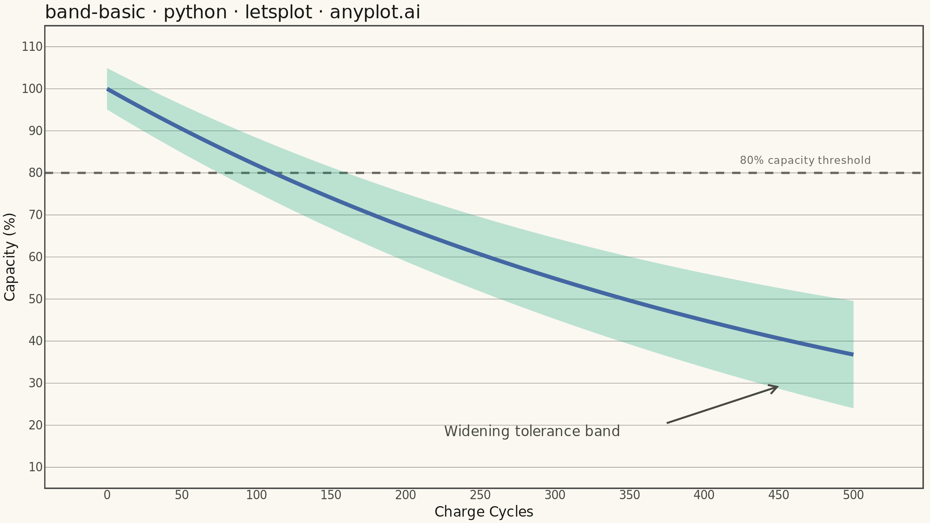
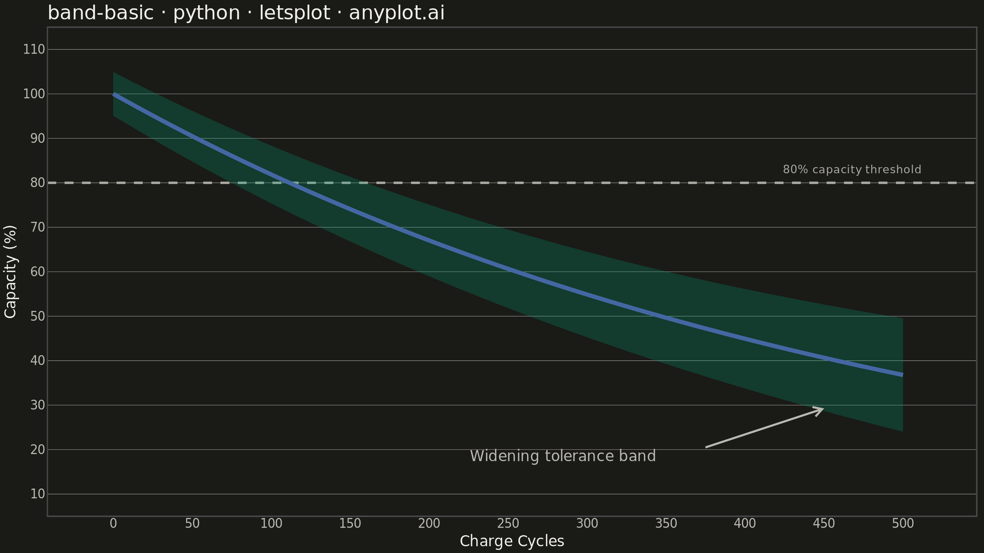
A band plot displays a filled region between two boundary lines, commonly used to show confidence intervals, prediction intervals, or ranges around a central trend line. The semi-transparent band provides visual representation of uncertainty or variability while maintaining visibility of underlying data or overlapping elements.
""" anyplot.ai
band-basic: Basic Band Plot
Library: letsplot 4.10.1 | Python 3.13.13
Quality: 88/100 | Updated: 2026-05-29
"""

import os

import numpy as np
import pandas as pd
from lets_plot import (
    LetsPlot,
    aes,
    arrow,
    element_blank,
    element_line,
    element_rect,
    element_text,
    geom_hline,
    geom_line,
    geom_ribbon,
    geom_segment,
    geom_text,
    ggplot,
    ggsave,
    ggsize,
    labs,
    scale_x_continuous,
    scale_y_continuous,
    theme,
    theme_minimal,
)


LetsPlot.setup_html()

# Theme tokens — Imprint palette, theme-adaptive chrome
THEME = os.getenv("ANYPLOT_THEME", "light")
PAGE_BG = "#FAF8F1" if THEME == "light" else "#1A1A17"
ELEVATED_BG = "#FFFDF6" if THEME == "light" else "#242420"
INK = "#1A1A17" if THEME == "light" else "#F0EFE8"
INK_SOFT = "#4A4A44" if THEME == "light" else "#B8B7B0"
INK_MUTED = "#6B6A63" if THEME == "light" else "#A8A79F"

IMPRINT_PALETTE = ["#009E73", "#C475FD", "#4467A3", "#BD8233", "#AE3030", "#2ABCCD", "#954477", "#99B314"]
BAND_FILL = IMPRINT_PALETTE[0]  # brand green — Imprint position 1
LINE_COLOR = IMPRINT_PALETTE[2]  # blue — Imprint position 3

# Data — battery capacity exponential decay over charge cycles (95% tolerance band)
cycles = np.linspace(0, 500, 100)
capacity_mean = 100 * np.exp(-0.002 * cycles)
tolerance = 2.5 + 0.008 * cycles
capacity_lower = capacity_mean - 1.96 * tolerance
capacity_upper = capacity_mean + 1.96 * tolerance

df = pd.DataFrame({"cycles": cycles, "mean": capacity_mean, "lower": capacity_lower, "upper": capacity_upper})

# Annotation — arrow pointing to widening lower band edge at cycle ~450
idx_450 = np.argmin(np.abs(cycles - 450))
annot_df = pd.DataFrame({"x": [285], "y": [18.5], "label": ["Widening tolerance band"]})
arrow_df = pd.DataFrame({"x": [375], "y": [20.5], "xend": [450], "yend": [float(capacity_lower[idx_450]) + 0.5]})

title = "band-basic · python · letsplot · anyplot.ai"

anyplot_theme = theme(
    plot_background=element_rect(fill=PAGE_BG, color=PAGE_BG),
    panel_background=element_rect(fill=PAGE_BG),
    panel_grid_major_x=element_blank(),
    panel_grid_major_y=element_line(color=INK_MUTED, size=0.3),
    panel_grid_minor=element_blank(),
    axis_title=element_text(size=12, color=INK),
    axis_text=element_text(size=10, color=INK_SOFT),
    axis_line_x=element_line(color=INK_SOFT),
    axis_line_y=element_blank(),
    plot_title=element_text(size=16, color=INK),
    legend_background=element_rect(fill=ELEVATED_BG),
    legend_text=element_text(size=10, color=INK_SOFT),
)

plot = (
    ggplot(df, aes(x="cycles"))
    + geom_hline(yintercept=80, color=INK_MUTED, size=0.8, linetype="dashed", tooltips="none")
    + geom_text(x=512, y=83, label="80% capacity threshold", size=4.5, color=INK_MUTED, hjust=1, tooltips="none")
    + geom_ribbon(aes(ymin="lower", ymax="upper"), fill=BAND_FILL, alpha=0.25, size=0)
    + geom_line(aes(y="mean"), color=LINE_COLOR, size=1.5)
    + geom_segment(
        aes(x="x", y="y", xend="xend", yend="yend"),
        data=arrow_df,
        color=INK_SOFT,
        size=0.7,
        arrow=arrow(length=8, type="open"),
        tooltips="none",
    )
    + geom_text(aes(x="x", y="y", label="label"), data=annot_df, size=6, color=INK_SOFT)
    + labs(x="Charge Cycles", y="Capacity (%)", title=title)
    + scale_x_continuous(limits=[-15, 520])
    + scale_y_continuous(limits=[10, 110])
    + theme_minimal()
    + anyplot_theme
    + ggsize(800, 450)
)

# Save
ggsave(plot, f"plot-{THEME}.png", path=".", scale=4)
ggsave(plot, f"plot-{THEME}.html", path=".")
Runnable source as JSON, for any HTTP client: https://api.anyplot.ai/specs/band-basic/letsplot/code. Any spec id and library id listed in llms-full.txt fit the same URL shape; every URL below is complete and callable.
{
  "spec_id": "band-basic",
  "language": "python",
  "library": "letsplot",
  "page": "https://anyplot.ai/band-basic/python/letsplot",
  "hub": "https://anyplot.ai/band-basic",
  "code_json": "https://api.anyplot.ai/specs/band-basic/letsplot/code",
  "spec_json": "https://api.anyplot.ai/specs/band-basic",
  "render_light_png": "https://storage.googleapis.com/anyplot-images/plots/band-basic/python/letsplot/plot-light.png",
  "render_dark_png": "https://storage.googleapis.com/anyplot-images/plots/band-basic/python/letsplot/plot-dark.png",
  "interactive_light_html": "https://storage.googleapis.com/anyplot-images/plots/band-basic/python/letsplot/plot-light.html",
  "interactive_dark_html": "https://storage.googleapis.com/anyplot-images/plots/band-basic/python/letsplot/plot-dark.html",
  "quality_score": 88.0,
  "license": "MIT",
  "guide": "https://anyplot.ai/llms.txt"
}
Part of Basic Band Plot on anyplot.ai.