The same plot in 14 other libraries — JavaScript: Chart.js, Apache ECharts, Highcharts, MUI X Charts; Python: Altair, Bokeh, lets-plot, Matplotlib, Plotly, plotnine, Pygal, Seaborn; R: ggplot2; Julia: Makie.jl. Compare all 15 side by side: Beer-Lambert Calibration Curve in Python, R, Julia and JavaScript.
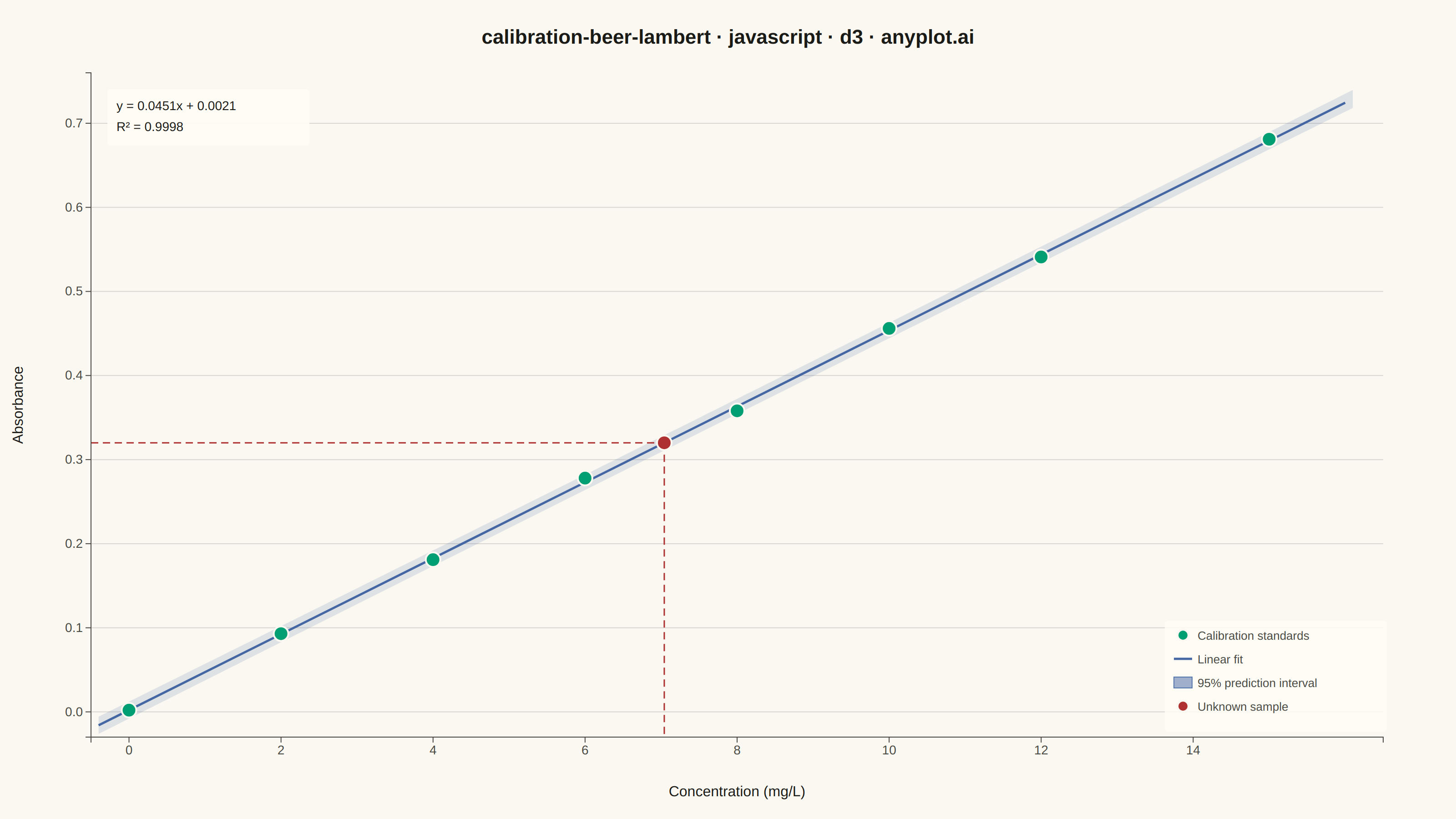
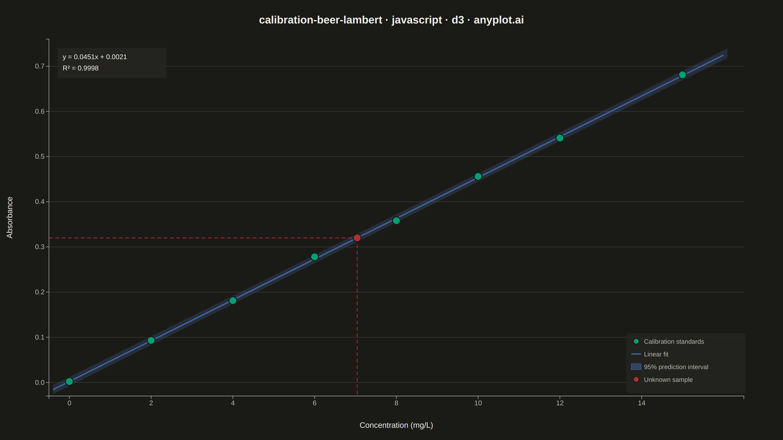
A calibration curve plotting absorbance versus concentration following Beer-Lambert law (A = εlc). Measured calibration standards are shown as scatter points with a linear regression fit line. The regression equation (y = mx + b) and R² value are displayed on the plot. An example unknown sample is marked with dashed lines extending to both axes, demonstrating how the curve is used to determine concentration from a measured absorbance. This plot is fundamental in analytical chemistry for quantitative spectrophotometric analysis.
// anyplot.ai
// calibration-beer-lambert: Beer-Lambert Calibration Curve
// Library: d3 7.9.0 | JavaScript 22.22.3
// Quality: 89/100 | Created: 2026-06-03

const t = window.ANYPLOT_TOKENS;
const theme = window.ANYPLOT_THEME;
const { width, height } = window.ANYPLOT_SIZE;
const margin = { top: 80, right: 80, bottom: 90, left: 100 };
const iw = width - margin.left - margin.right;
const ih = height - margin.top - margin.bottom;

// --- Data: UV-Vis spectrophotometry calibration standards (blank + 7 levels) ---
const calibData = [
  { conc: 0,  abs: 0.002 },
  { conc: 2,  abs: 0.093 },
  { conc: 4,  abs: 0.181 },
  { conc: 6,  abs: 0.278 },
  { conc: 8,  abs: 0.358 },
  { conc: 10, abs: 0.456 },
  { conc: 12, abs: 0.541 },
  { conc: 15, abs: 0.681 },
];
const unknownAbs = 0.320;

// --- Linear regression (ordinary least squares) ---
const n     = calibData.length;
const sumX  = calibData.reduce((s, d) => s + d.conc, 0);
const sumY  = calibData.reduce((s, d) => s + d.abs,  0);
const sumXY = calibData.reduce((s, d) => s + d.conc * d.abs, 0);
const sumX2 = calibData.reduce((s, d) => s + d.conc * d.conc, 0);
const xMean = sumX / n;
const yMean = sumY / n;
const Sxx       = sumX2 - (sumX * sumX) / n;
const slope     = (sumXY - (sumX * sumY) / n) / Sxx;
const intercept = yMean - slope * xMean;

const ssTot = calibData.reduce((s, d) => s + (d.abs - yMean) ** 2, 0);
const ssRes = calibData.reduce((s, d) => s + (d.abs - (slope * d.conc + intercept)) ** 2, 0);
const r2    = 1 - ssRes / ssTot;

// 95% prediction interval — t-critical for df = n − 2 = 6 is 2.447
const se    = Math.sqrt(ssRes / (n - 2));
const tCrit = 2.447;
const unknownConc = (unknownAbs - intercept) / slope;

// Band opacity adapts to theme — dark background needs stronger fill for visibility
const bandOpacity = theme === "dark" ? 0.25 : 0.15;

// --- Scales ---
const xScale = d3.scaleLinear().domain([-0.5, 16.5]).range([0, iw]);
const yScale = d3.scaleLinear().domain([-0.03, 0.76]).range([ih, 0]);

// --- Prediction band data (sampled at fine intervals) ---
const bandPts = d3.range(-0.4, 16.15, 0.1).map(x => {
  const yHat = slope * x + intercept;
  const hw   = tCrit * se * Math.sqrt(1 + 1 / n + (x - xMean) ** 2 / Sxx);
  return { x, lo: yHat - hw, hi: yHat + hw };
});

// --- SVG ---
const svg = d3.select("#container")
  .append("svg")
  .attr("width", width)
  .attr("height", height);
const g = svg.append("g").attr("transform", `translate(${margin.left},${margin.top})`);

// --- Y-axis gridlines (behind everything) — D3 data join ---
g.selectAll(".ygrid")
  .data([0, 0.1, 0.2, 0.3, 0.4, 0.5, 0.6, 0.7])
  .join("line")
  .attr("class", "ygrid")
  .attr("x1", 0).attr("x2", iw)
  .attr("y1", v => yScale(v)).attr("y2", v => yScale(v))
  .attr("stroke", t.grid).attr("stroke-width", 1);

// --- Prediction interval band ---
g.append("path")
  .datum(bandPts)
  .attr("d", d3.area()
    .x(d => xScale(d.x))
    .y0(d => yScale(d.lo))
    .y1(d => yScale(d.hi)))
  .attr("fill", t.palette[2])
  .attr("opacity", bandOpacity);

// --- Regression line (d3.line path generator — more idiomatic than SVG <line>) ---
g.append("path")
  .datum([[-0.4, slope * -0.4 + intercept], [16.0, slope * 16.0 + intercept]])
  .attr("d", d3.line().x(d => xScale(d[0])).y(d => yScale(d[1])))
  .attr("stroke", t.palette[2])
  .attr("stroke-width", 2.5)
  .attr("fill", "none");

// --- Unknown sample dashed guide lines ---
// Horizontal: y-axis edge → unknown point (shows measured absorbance)
g.append("line")
  .attr("x1", 0).attr("y1", yScale(unknownAbs))
  .attr("x2", xScale(unknownConc)).attr("y2", yScale(unknownAbs))
  .attr("stroke", t.palette[4]).attr("stroke-width", 1.5)
  .attr("stroke-dasharray", "8,5");

// Vertical: unknown point → x-axis (shows determined concentration)
g.append("line")
  .attr("x1", xScale(unknownConc)).attr("y1", yScale(unknownAbs))
  .attr("x2", xScale(unknownConc)).attr("y2", ih)
  .attr("stroke", t.palette[4]).attr("stroke-width", 1.5)
  .attr("stroke-dasharray", "8,5");

// --- Calibration data points ---
g.selectAll(".std")
  .data(calibData)
  .join("circle")
  .attr("class", "std")
  .attr("cx", d => xScale(d.conc))
  .attr("cy", d => yScale(d.abs))
  .attr("r", 8)
  .attr("fill", t.palette[0])
  .attr("stroke", t.pageBg)
  .attr("stroke-width", 2);

// --- Unknown sample point ---
g.append("circle")
  .attr("cx", xScale(unknownConc))
  .attr("cy", yScale(unknownAbs))
  .attr("r", 8)
  .attr("fill", t.palette[4])
  .attr("stroke", t.pageBg)
  .attr("stroke-width", 2);

// --- Axes ---
const xAx = g.append("g")
  .attr("transform", `translate(0,${ih})`)
  .call(d3.axisBottom(xScale).tickValues([0, 2, 4, 6, 8, 10, 12, 14]));
const yAx = g.append("g")
  .call(d3.axisLeft(yScale).tickValues([0, 0.1, 0.2, 0.3, 0.4, 0.5, 0.6, 0.7]));

for (const ax of [xAx, yAx]) {
  ax.selectAll("text").attr("fill", t.inkSoft).style("font-size", "14px");
  ax.selectAll(".tick line").attr("stroke", t.inkSoft);
  ax.select(".domain").attr("stroke", t.inkSoft);
}

// --- Axis labels ---
g.append("text")
  .attr("x", iw / 2).attr("y", ih + 65)
  .attr("text-anchor", "middle")
  .attr("fill", t.ink)
  .style("font-size", "16px")
  .text("Concentration (mg/L)");

g.append("text")
  .attr("transform", "rotate(-90)")
  .attr("x", -(ih / 2)).attr("y", -75)
  .attr("text-anchor", "middle")
  .attr("fill", t.ink)
  .style("font-size", "16px")
  .text("Absorbance");

// --- Equation annotation box (upper-left, above data region) ---
const eqSign = intercept >= 0 ? "+" : "−";
const eqAbsInt = Math.abs(intercept).toFixed(4);
const ax0 = 18, ay0 = 18;
g.append("rect")
  .attr("x", ax0).attr("y", ay0)
  .attr("width", 222).attr("height", 62)
  .attr("fill", t.elevatedBg).attr("rx", 4).attr("opacity", 0.92);
g.append("text")
  .attr("x", ax0 + 10).attr("y", ay0 + 23)
  .attr("fill", t.ink).style("font-size", "14px")
  .text(`y = ${slope.toFixed(4)}x ${eqSign} ${eqAbsInt}`);
g.append("text")
  .attr("x", ax0 + 10).attr("y", ay0 + 46)
  .attr("fill", t.ink).style("font-size", "14px")
  .text(`R² = ${r2.toFixed(4)}`);

// --- Legend (lower-right, clear of data) ---
const lx = iw - 230, ly = ih - 118;
const legendItems = [
  { type: "dot",  color: t.palette[0], label: "Calibration standards" },
  { type: "line", color: t.palette[2], label: "Linear fit" },
  { type: "band", color: t.palette[2], label: "95% prediction interval" },
  { type: "dot",  color: t.palette[4], label: "Unknown sample" },
];

// Subtle legend background for visual polish
g.append("rect")
  .attr("x", lx - 10).attr("y", ly - 10)
  .attr("width", 244).attr("height", legendItems.length * 26 + 18)
  .attr("fill", t.elevatedBg).attr("rx", 4).attr("opacity", 0.85);

legendItems.forEach((item, i) => {
  const iy = ly + i * 26;
  if (item.type === "dot") {
    g.append("circle")
      .attr("cx", lx + 10).attr("cy", iy + 6).attr("r", 6)
      .attr("fill", item.color).attr("stroke", t.pageBg).attr("stroke-width", 2);
  } else if (item.type === "line") {
    g.append("line")
      .attr("x1", lx).attr("y1", iy + 6)
      .attr("x2", lx + 20).attr("y2", iy + 6)
      .attr("stroke", item.color).attr("stroke-width", 2.5);
  } else {
    // Band swatch: elevated opacity + outline stroke for dark-theme readability
    g.append("rect")
      .attr("x", lx).attr("y", iy)
      .attr("width", 20).attr("height", 12)
      .attr("fill", item.color).attr("opacity", 0.5);
    g.append("rect")
      .attr("x", lx).attr("y", iy)
      .attr("width", 20).attr("height", 12)
      .attr("fill", "none")
      .attr("stroke", item.color).attr("stroke-width", 1).attr("opacity", 0.85);
  }
  g.append("text")
    .attr("x", lx + 26).attr("y", iy + 11)
    .attr("fill", t.inkSoft).style("font-size", "13px")
    .text(item.label);
});

// --- Title ---
svg.append("text")
  .attr("x", width / 2).attr("y", 48)
  .attr("text-anchor", "middle")
  .attr("fill", t.ink)
  .style("font-size", "22px").style("font-weight", "600")
  .text("calibration-beer-lambert · javascript · d3 · anyplot.ai");
Runnable source as JSON, for any HTTP client: https://api.anyplot.ai/specs/calibration-beer-lambert/d3/code. Any spec id and library id listed in llms-full.txt fit the same URL shape; every URL below is complete and callable.
{
  "spec_id": "calibration-beer-lambert",
  "language": "javascript",
  "library": "d3",
  "page": "https://anyplot.ai/calibration-beer-lambert/javascript/d3",
  "hub": "https://anyplot.ai/calibration-beer-lambert",
  "code_json": "https://api.anyplot.ai/specs/calibration-beer-lambert/d3/code",
  "spec_json": "https://api.anyplot.ai/specs/calibration-beer-lambert",
  "render_light_png": "https://storage.googleapis.com/anyplot-images/plots/calibration-beer-lambert/javascript/d3/plot-light.png",
  "render_dark_png": "https://storage.googleapis.com/anyplot-images/plots/calibration-beer-lambert/javascript/d3/plot-dark.png",
  "interactive_light_html": "https://storage.googleapis.com/anyplot-images/plots/calibration-beer-lambert/javascript/d3/plot-light.html",
  "interactive_dark_html": "https://storage.googleapis.com/anyplot-images/plots/calibration-beer-lambert/javascript/d3/plot-dark.html",
  "quality_score": 89.0,
  "license": "MIT",
  "guide": "https://anyplot.ai/llms.txt"
}
Part of Beer-Lambert Calibration Curve on anyplot.ai.