The same plot in 14 other libraries — JavaScript: Chart.js, D3.js, Highcharts, MUI X Charts; Python: Altair, Bokeh, lets-plot, Matplotlib, Plotly, plotnine, Pygal, Seaborn; R: ggplot2; Julia: Makie.jl. Compare all 15 side by side: Beer-Lambert Calibration Curve in Python, R, Julia and JavaScript.
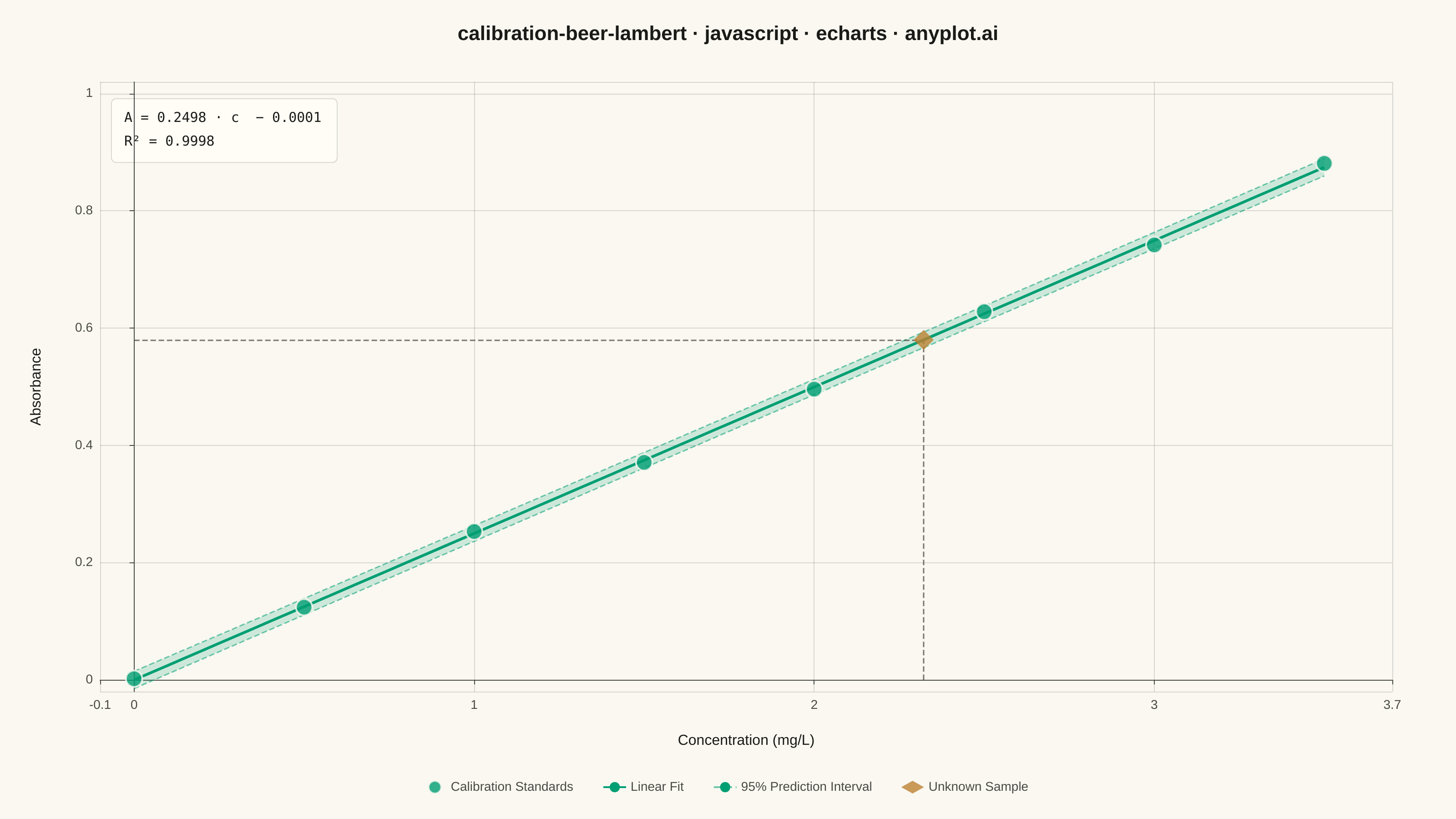
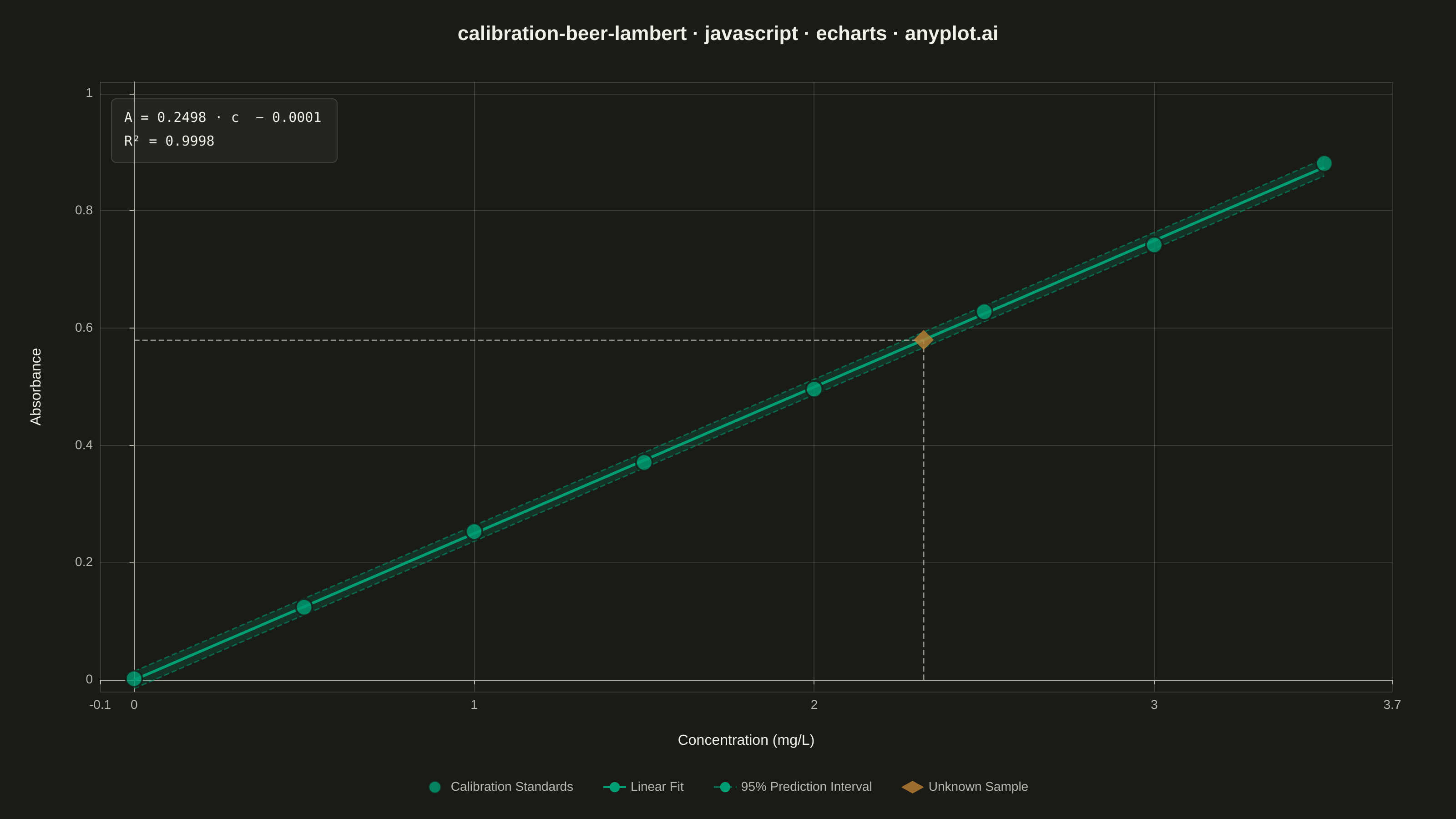
A calibration curve plotting absorbance versus concentration following Beer-Lambert law (A = εlc). Measured calibration standards are shown as scatter points with a linear regression fit line. The regression equation (y = mx + b) and R² value are displayed on the plot. An example unknown sample is marked with dashed lines extending to both axes, demonstrating how the curve is used to determine concentration from a measured absorbance. This plot is fundamental in analytical chemistry for quantitative spectrophotometric analysis.
// anyplot.ai
// calibration-beer-lambert: Beer-Lambert Calibration Curve
// Library: echarts 5.5.1 | JavaScript 22.22.3
// Quality: 92/100 | Created: 2026-06-03

//# anyplot-orientation: landscape

const t = window.ANYPLOT_TOKENS;

// --- Data (hardcoded, deterministic) ---
// UV-Vis spectrophotometry standards for a dye solution at 520 nm
const stdConc = [0,     0.5,   1.0,   1.5,   2.0,   2.5,   3.0,   3.5];
const stdAbs  = [0.002, 0.124, 0.253, 0.371, 0.496, 0.628, 0.742, 0.881];
const n = stdConc.length;

// Linear regression: A = m·c + b (Beer-Lambert law)
let sumX = 0, sumY = 0, sumXX = 0, sumXY = 0;
for (let i = 0; i < n; i++) {
  sumX  += stdConc[i];
  sumY  += stdAbs[i];
  sumXX += stdConc[i] * stdConc[i];
  sumXY += stdConc[i] * stdAbs[i];
}
const slope     = (n * sumXY - sumX * sumY) / (n * sumXX - sumX * sumX);
const intercept = (sumY - slope * sumX) / n;
const xMean     = sumX / n;
const Sxx       = sumXX - sumX * sumX / n;
const yMean     = sumY / n;
const SStot     = stdAbs.reduce((s, y) => s + (y - yMean) ** 2, 0);
const SSres     = stdConc.reduce((s, x, i) => s + (stdAbs[i] - (slope * x + intercept)) ** 2, 0);
const r2        = 1 - SSres / SStot;
const se        = Math.sqrt(SSres / (n - 2));
const tCrit     = 2.447; // t_{0.975}, 6 df

// Regression line + 95% prediction interval over the concentration range
const nFit   = 71;
const xFit   = Array.from({ length: nFit }, (_, i) => i * 3.5 / (nFit - 1));
const piHalf = xFit.map(x => tCrit * se * Math.sqrt(1 + 1 / n + (x - xMean) ** 2 / Sxx));
const regLine = xFit.map(x => [x, slope * x + intercept]);
const piUpper = xFit.map((x, i) => [x, slope * x + intercept + piHalf[i]]);
const piLower = xFit.map((x, i) => [x, slope * x + intercept - piHalf[i]]);

// Unknown sample: measured absorbance → inferred concentration
const unknownAbs  = 0.580;
const unknownConc = (unknownAbs - intercept) / slope;

// Equation annotation strings
const signStr = intercept >= 0 ? `+ ${intercept.toFixed(4)}` : `− ${Math.abs(intercept).toFixed(4)}`;
const eqText  = `A = ${slope.toFixed(4)} · c  ${signStr}`;
const r2Text  = `R² = ${r2.toFixed(4)}`;

// --- Init ---
const chart = echarts.init(document.getElementById("container"));

const bandColor = 'rgba(0,158,115,0.18)';

// Base option (PI dashed boundary lines + data series)
chart.setOption({
  animation: false,
  color: t.palette,
  backgroundColor: 'transparent',
  title: {
    text: 'calibration-beer-lambert · javascript · echarts · anyplot.ai',
    left: 'center',
    top: 22,
    textStyle: { color: t.ink, fontSize: 22, fontWeight: 'bold' }
  },
  legend: {
    data: ['Calibration Standards', 'Linear Fit', '95% Prediction Interval', 'Unknown Sample'],
    bottom: 22,
    itemGap: 32,
    textStyle: { color: t.inkSoft, fontSize: 14 }
  },
  grid: { left: 110, right: 70, top: 90, bottom: 140 },
  xAxis: {
    type: 'value',
    name: 'Concentration (mg/L)',
    nameLocation: 'middle',
    nameGap: 46,
    nameTextStyle: { color: t.ink, fontSize: 16 },
    min: -0.1,
    max: 3.7,
    axisLabel: { color: t.inkSoft, fontSize: 14 },
    axisLine:  { show: true, lineStyle: { color: t.inkSoft } },
    axisTick:  { lineStyle: { color: t.inkSoft } },
    splitLine: { lineStyle: { color: t.grid } }
  },
  yAxis: {
    type: 'value',
    name: 'Absorbance',
    nameLocation: 'middle',
    nameGap: 62,
    nameTextStyle: { color: t.ink, fontSize: 16 },
    min: -0.02,
    max: 1.02,
    axisLabel: { color: t.inkSoft, fontSize: 14 },
    axisLine:  { show: true, lineStyle: { color: t.inkSoft } },
    axisTick:  { lineStyle: { color: t.inkSoft } },
    splitLine: { lineStyle: { color: t.grid } }
  },
  series: [
    // PI upper boundary (dashed line, defines the legend entry)
    {
      name: '95% Prediction Interval',
      type: 'line',
      data: piUpper,
      lineStyle: { color: t.palette[0], width: 1.5, type: 'dashed', opacity: 0.55 },
      symbol: 'none',
      silent: true,
      z: 2
    },
    // PI lower boundary (dashed line, shares legend entry via same name)
    {
      name: '95% Prediction Interval',
      type: 'line',
      data: piLower,
      lineStyle: { color: t.palette[0], width: 1.5, type: 'dashed', opacity: 0.55 },
      symbol: 'none',
      silent: true,
      z: 2
    },
    // Regression line
    {
      name: 'Linear Fit',
      type: 'line',
      data: regLine,
      color: t.palette[0],
      lineStyle: { color: t.palette[0], width: 3 },
      symbol: 'none',
      z: 3
    },
    // Calibration standard points
    {
      name: 'Calibration Standards',
      type: 'scatter',
      data: stdConc.map((c, i) => [c, stdAbs[i]]),
      symbolSize: 18,
      itemStyle: { color: t.palette[0], borderColor: t.pageBg, borderWidth: 2 },
      z: 4
    },
    // Unknown sample with dashed guide lines to axes
    {
      name: 'Unknown Sample',
      type: 'scatter',
      data: [[unknownConc, unknownAbs]],
      symbol: 'diamond',
      symbolSize: 22,
      itemStyle: { color: t.palette[3] },
      z: 5,
      markLine: {
        symbol: ['none', 'none'],
        animation: false,
        lineStyle: { type: 'dashed', color: t.inkSoft, width: 1.5, opacity: 0.75 },
        label: { show: false },
        data: [
          [{ coord: [0, unknownAbs] },  { coord: [unknownConc, unknownAbs] }],
          [{ coord: [unknownConc, 0] }, { coord: [unknownConc, unknownAbs] }]
        ]
      }
    }
  ]
});

// Add the PI filled polygon + equation box via convertToPixel (runs after layout is set)
const upperPx = piUpper.map(pt => chart.convertToPixel('grid', pt));
const lowerPx = piLower.map(pt => chart.convertToPixel('grid', pt));
const bandPoly = [...upperPx, ...[...lowerPx].reverse()];

chart.setOption({
  graphic: [
    // PI filled band polygon
    {
      type: 'polygon',
      shape: { points: bandPoly },
      style: { fill: bandColor, stroke: 'none' },
      silent: true,
      z: 1
    },
    // Equation annotation box
    {
      type: 'group',
      left: 122,
      top: 108,
      children: [
        {
          type: 'rect',
          shape: { x: 0, y: 0, width: 248, height: 70, r: 5 },
          style: { fill: t.elevatedBg, stroke: t.grid, lineWidth: 1 }
        },
        {
          type: 'text',
          x: 14,
          y: 14,
          style: { text: eqText, fill: t.ink, fontSize: 15, fontFamily: 'monospace' }
        },
        {
          type: 'text',
          x: 14,
          y: 40,
          style: { text: r2Text, fill: t.ink, fontSize: 15, fontFamily: 'monospace' }
        }
      ]
    }
  ]
});
Runnable source as JSON, for any HTTP client: https://api.anyplot.ai/specs/calibration-beer-lambert/echarts/code. Any spec id and library id listed in llms-full.txt fit the same URL shape; every URL below is complete and callable.
{
  "spec_id": "calibration-beer-lambert",
  "language": "javascript",
  "library": "echarts",
  "page": "https://anyplot.ai/calibration-beer-lambert/javascript/echarts",
  "hub": "https://anyplot.ai/calibration-beer-lambert",
  "code_json": "https://api.anyplot.ai/specs/calibration-beer-lambert/echarts/code",
  "spec_json": "https://api.anyplot.ai/specs/calibration-beer-lambert",
  "render_light_png": "https://storage.googleapis.com/anyplot-images/plots/calibration-beer-lambert/javascript/echarts/plot-light.png",
  "render_dark_png": "https://storage.googleapis.com/anyplot-images/plots/calibration-beer-lambert/javascript/echarts/plot-dark.png",
  "interactive_light_html": "https://storage.googleapis.com/anyplot-images/plots/calibration-beer-lambert/javascript/echarts/plot-light.html",
  "interactive_dark_html": "https://storage.googleapis.com/anyplot-images/plots/calibration-beer-lambert/javascript/echarts/plot-dark.html",
  "quality_score": 92.0,
  "license": "MIT",
  "guide": "https://anyplot.ai/llms.txt"
}
Part of Beer-Lambert Calibration Curve on anyplot.ai.