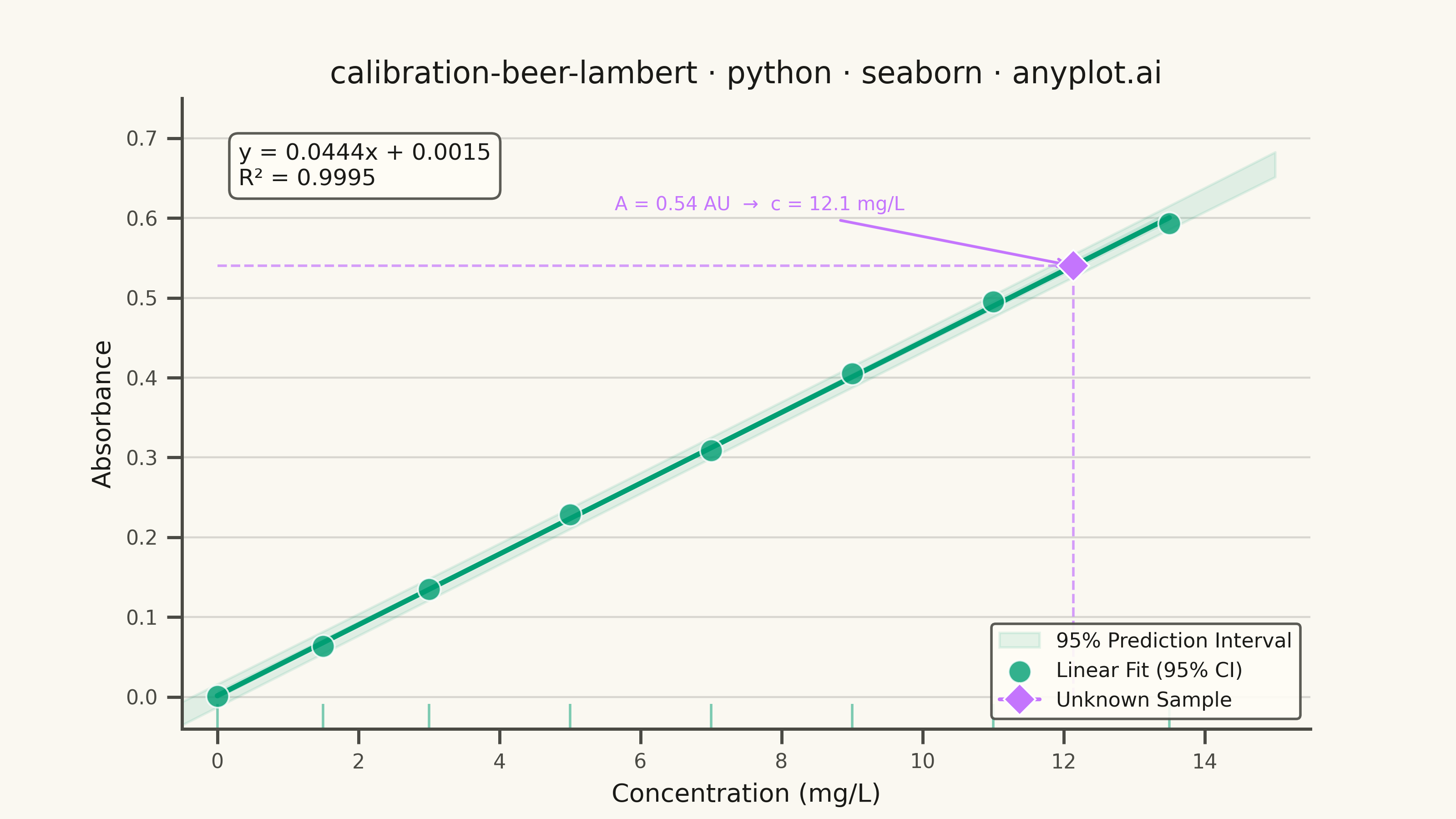
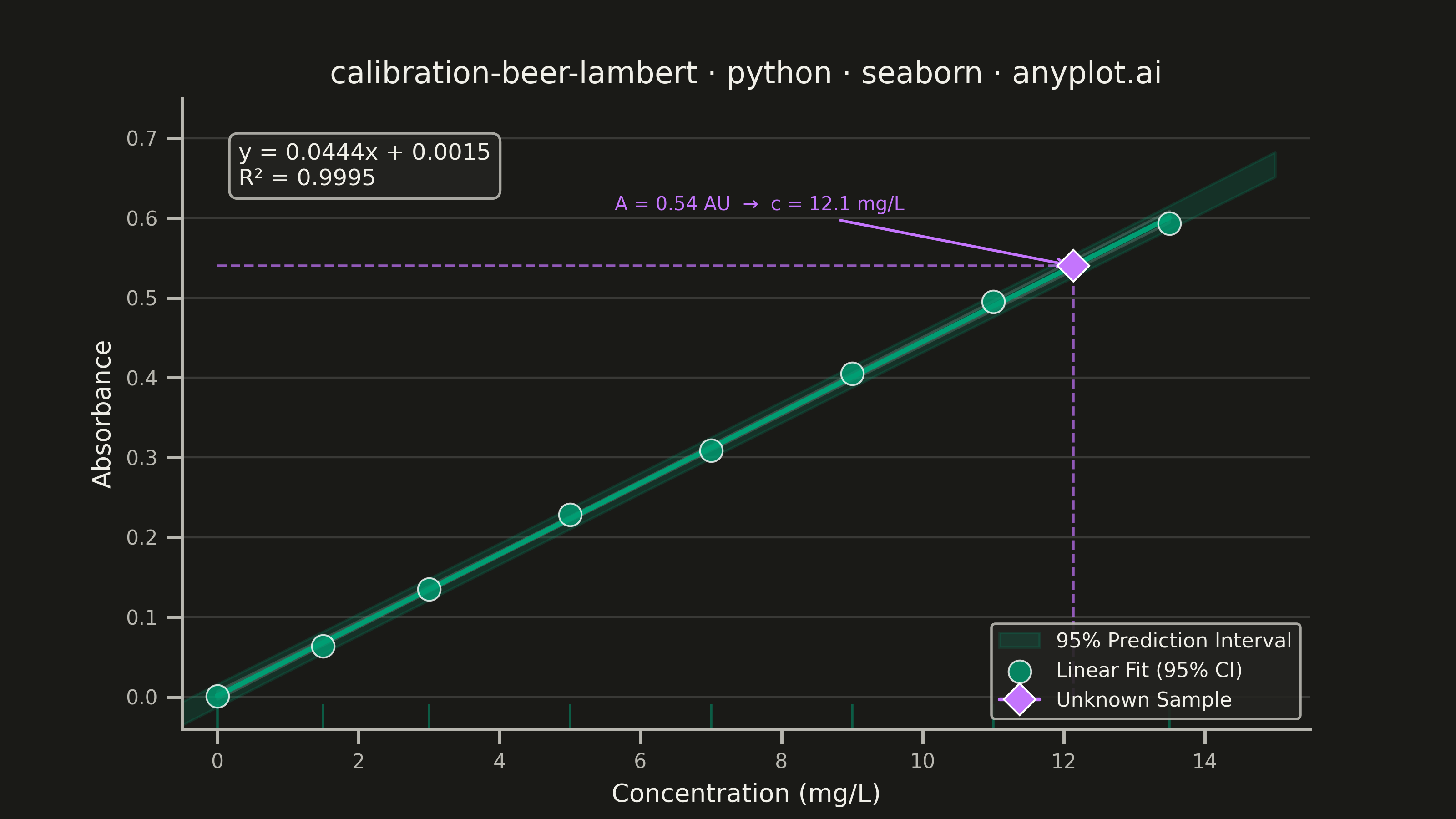
A calibration curve plotting absorbance versus concentration following Beer-Lambert law (A = εlc). Measured calibration standards are shown as scatter points with a linear regression fit line. The regression equation (y = mx + b) and R² value are displayed on the plot. An example unknown sample is marked with dashed lines extending to both axes, demonstrating how the curve is used to determine concentration from a measured absorbance. This plot is fundamental in analytical chemistry for quantitative spectrophotometric analysis.
""" anyplot.ai
calibration-beer-lambert: Beer-Lambert Calibration Curve
Library: seaborn 0.13.2 | Python 3.13.13
Quality: 90/100 | Updated: 2026-06-03
"""

import os

import matplotlib.pyplot as plt
import numpy as np
import pandas as pd
import seaborn as sns
from scipy import stats


THEME = os.getenv("ANYPLOT_THEME", "light")
PAGE_BG = "#FAF8F1" if THEME == "light" else "#1A1A17"
ELEVATED_BG = "#FFFDF6" if THEME == "light" else "#242420"
INK = "#1A1A17" if THEME == "light" else "#F0EFE8"
INK_SOFT = "#4A4A44" if THEME == "light" else "#B8B7B0"
PI_ALPHA = 0.18 if THEME == "dark" else 0.10  # more visible against near-black background

# Imprint palette — brand green always first
IMPRINT_PALETTE = ["#009E73", "#C475FD", "#4467A3", "#BD8233", "#AE3030", "#2ABCCD", "#954477", "#99B314"]
BRAND = IMPRINT_PALETTE[0]
SECOND = IMPRINT_PALETTE[1]

sns.set_theme(
    style="ticks",
    rc={
        "figure.facecolor": PAGE_BG,
        "axes.facecolor": PAGE_BG,
        "axes.edgecolor": INK_SOFT,
        "axes.labelcolor": INK,
        "text.color": INK,
        "xtick.color": INK_SOFT,
        "ytick.color": INK_SOFT,
        "grid.color": INK,
        "grid.alpha": 0.15,
        "legend.facecolor": ELEVATED_BG,
        "legend.edgecolor": INK_SOFT,
    },
)

# Data — varied standard set to distinguish from sibling implementations
np.random.seed(7)
concentrations = np.array([0.0, 1.5, 3.0, 5.0, 7.0, 9.0, 11.0, 13.5])
epsilon_l = 0.045
true_absorbance = epsilon_l * concentrations
measured_absorbance = true_absorbance + np.random.normal(0, 0.008, len(concentrations))
measured_absorbance[0] = 0.001  # blank near zero

df = pd.DataFrame({"Concentration (mg/L)": concentrations, "Absorbance": measured_absorbance})

# Linear regression
slope, intercept, r_value, _, _ = stats.linregress(concentrations, measured_absorbance)
r_squared = r_value**2

# Prediction interval (wider than CI, spec-required)
n = len(concentrations)
x_mean = np.mean(concentrations)
fit_x = np.linspace(-0.5, 15.0, 200)
fit_y = slope * fit_x + intercept
residuals = measured_absorbance - (slope * concentrations + intercept)
se_pred = np.sqrt(
    (np.sum(residuals**2) / (n - 2)) * (1 + 1 / n + (fit_x - x_mean) ** 2 / np.sum((concentrations - x_mean) ** 2))
)
t_crit = stats.t.ppf(0.975, df=n - 2)
pred_upper = fit_y + t_crit * se_pred
pred_lower = fit_y - t_crit * se_pred

# Unknown sample at a different location from sibling implementations (~12 mg/L)
unknown_absorbance = 0.54
unknown_concentration = (unknown_absorbance - intercept) / slope

# Canvas: landscape 3200×1800 px — figsize × dpi, no bbox_inches='tight'
fig, ax = plt.subplots(figsize=(8, 4.5), dpi=400)

# Prediction interval band (alpha theme-adaptive for dark-bg visibility)
ax.fill_between(fit_x, pred_lower, pred_upper, color=BRAND, alpha=PI_ALPHA, label="95% Prediction Interval")

# Scatter + regression line with 95% CI via regplot
sns.regplot(
    data=df,
    x="Concentration (mg/L)",
    y="Absorbance",
    ax=ax,
    ci=95,
    color=BRAND,
    scatter_kws={"s": 80, "edgecolor": "white", "linewidths": 0.7, "zorder": 5},
    line_kws={"linewidth": 2.0, "zorder": 4},
    label="Linear Fit (95% CI)",
)

# Rug ticks showing calibration standard positions along concentration axis
sns.rugplot(x=concentrations, height=0.04, color=BRAND, alpha=0.5, expand_margins=False, ax=ax)

# Unknown sample marker
ax.plot(
    unknown_concentration,
    unknown_absorbance,
    marker="D",
    markersize=9,
    color=SECOND,
    markeredgecolor="white",
    markeredgewidth=0.7,
    zorder=6,
    label="Unknown Sample",
)

# Dashed projection lines to axes
ax.plot(
    [unknown_concentration, unknown_concentration],
    [0, unknown_absorbance],
    linestyle="--",
    color=SECOND,
    linewidth=1.0,
    alpha=0.7,
)
ax.plot(
    [0, unknown_concentration],
    [unknown_absorbance, unknown_absorbance],
    linestyle="--",
    color=SECOND,
    linewidth=1.0,
    alpha=0.7,
)

# Regression equation annotation
eq_text = f"y = {slope:.4f}x + {intercept:.4f}\nR² = {r_squared:.4f}"
ax.text(
    0.05,
    0.93,
    eq_text,
    transform=ax.transAxes,
    fontsize=9,
    verticalalignment="top",
    color=INK,
    bbox={"boxstyle": "round,pad=0.4", "facecolor": ELEVATED_BG, "edgecolor": INK_SOFT, "alpha": 0.9},
)

# Unknown sample annotation — shows interpolation direction explicitly (storytelling)
ax.annotate(
    f"A = {unknown_absorbance:.2f} AU  →  c = {unknown_concentration:.1f} mg/L",
    xy=(unknown_concentration, unknown_absorbance),
    xytext=(unknown_concentration - 6.5, unknown_absorbance + 0.07),
    fontsize=7.5,
    color=SECOND,
    arrowprops={"arrowstyle": "->", "color": SECOND, "lw": 1.1},
)

ax.set_xlabel("Concentration (mg/L)", fontsize=10)
ax.set_ylabel("Absorbance", fontsize=10)
ax.set_title("calibration-beer-lambert · python · seaborn · anyplot.ai", fontsize=12, fontweight="medium", color=INK)
ax.tick_params(axis="both", labelsize=8, labelcolor=INK_SOFT)
ax.yaxis.grid(True, alpha=0.15, linewidth=0.8, color=INK)
ax.set_xlim(-0.5, 15.5)
ax.set_ylim(-0.04, 0.75)
ax.legend(fontsize=8, loc="lower right", framealpha=0.9)
sns.despine(ax=ax)

plt.savefig(f"plot-{THEME}.png", dpi=400, facecolor=PAGE_BG)
Runnable source as JSON, for any HTTP client: https://api.anyplot.ai/specs/calibration-beer-lambert/seaborn/code. Any spec id and library id listed in llms-full.txt fit the same URL shape; every URL below is complete and callable.
{
  "spec_id": "calibration-beer-lambert",
  "language": "python",
  "library": "seaborn",
  "page": "https://anyplot.ai/calibration-beer-lambert/python/seaborn",
  "hub": "https://anyplot.ai/calibration-beer-lambert",
  "code_json": "https://api.anyplot.ai/specs/calibration-beer-lambert/seaborn/code",
  "spec_json": "https://api.anyplot.ai/specs/calibration-beer-lambert",
  "render_light_png": "https://storage.googleapis.com/anyplot-images/plots/calibration-beer-lambert/python/seaborn/plot-light.png",
  "render_dark_png": "https://storage.googleapis.com/anyplot-images/plots/calibration-beer-lambert/python/seaborn/plot-dark.png",
  "quality_score": 90.0,
  "license": "MIT",
  "guide": "https://anyplot.ai/llms.txt"
}
Part of Beer-Lambert Calibration Curve on anyplot.ai.