The same plot in 14 other libraries — JavaScript: Chart.js, D3.js, Apache ECharts, Highcharts; Python: Altair, Bokeh, lets-plot, Matplotlib, Plotly, plotnine, Pygal, Seaborn; R: ggplot2; Julia: Makie.jl. Compare all 15 side by side: Beer-Lambert Calibration Curve in Python, R, Julia and JavaScript.
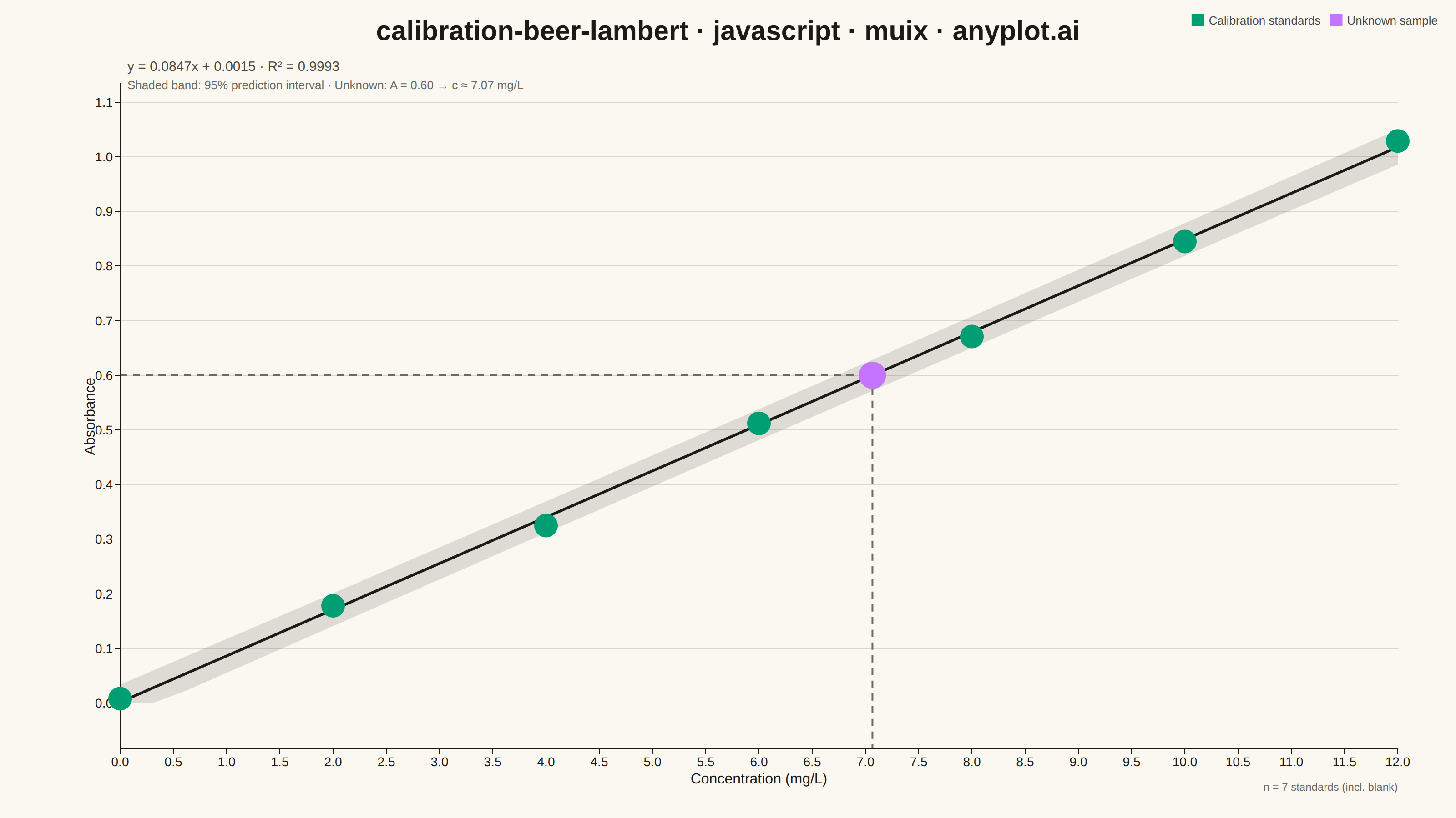
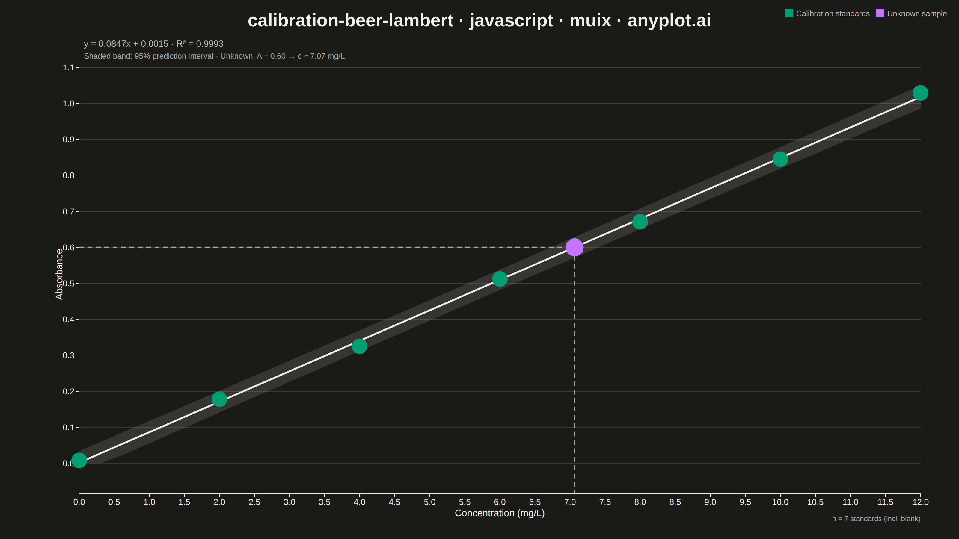
A calibration curve plotting absorbance versus concentration following Beer-Lambert law (A = εlc). Measured calibration standards are shown as scatter points with a linear regression fit line. The regression equation (y = mx + b) and R² value are displayed on the plot. An example unknown sample is marked with dashed lines extending to both axes, demonstrating how the curve is used to determine concentration from a measured absorbance. This plot is fundamental in analytical chemistry for quantitative spectrophotometric analysis.
// anyplot.ai
// calibration-beer-lambert: Beer-Lambert Calibration Curve
// Library: muix 7.29.1 | JavaScript 22.23.2
// Quality: 91/100 | Created: 2026-08-20
import { ChartContainer } from "@mui/x-charts/ChartContainer";
import { ScatterPlot } from "@mui/x-charts/ScatterChart";
import { LinePlot } from "@mui/x-charts/LineChart";
import { ChartsXAxis } from "@mui/x-charts/ChartsXAxis";
import { ChartsYAxis } from "@mui/x-charts/ChartsYAxis";
import { ChartsGrid } from "@mui/x-charts/ChartsGrid";
import { ChartsLegend } from "@mui/x-charts/ChartsLegend";
import { useXScale, useYScale, useDrawingArea } from "@mui/x-charts/hooks";

const t = window.ANYPLOT_TOKENS;
const THEME = window.ANYPLOT_THEME === "dark" ? "dark" : "light";
// ANYPLOT_TOKENS has no "muted" anchor — derive it from default-style-guide.md
// "Theme-adaptive Chrome" (tertiary text / confidence-band fill token).
const INK_MUTED = THEME === "dark" ? "#A8A79F" : "#6B6A63";

// --- Data: UV-Vis calibration standards for a drug-substance assay (243 nm) -
// Blank plus six standards spanning the assay's working range.
const concentration = [0, 2, 4, 6, 8, 10, 12]; // mg/L
const absorbance = [0.008, 0.178, 0.325, 0.512, 0.671, 0.845, 1.029]; // dimensionless

// --- Ordinary least-squares fit (Beer-Lambert: A = εlc, i.e. y = mx + b) ----
const n = concentration.length;
const xMean = concentration.reduce((a, b) => a + b, 0) / n;
const yMean = absorbance.reduce((a, b) => a + b, 0) / n;
let sxy = 0;
let sxx = 0;
for (let i = 0; i < n; i += 1) {
  sxy += (concentration[i] - xMean) * (absorbance[i] - yMean);
  sxx += (concentration[i] - xMean) ** 2;
}
const slope = sxy / sxx;
const intercept = yMean - slope * xMean;

let ssRes = 0;
let ssTot = 0;
for (let i = 0; i < n; i += 1) {
  const fitted = intercept + slope * concentration[i];
  ssRes += (absorbance[i] - fitted) ** 2;
  ssTot += (absorbance[i] - yMean) ** 2;
}
const rSquared = 1 - ssRes / ssTot;
const residualStdErr = Math.sqrt(ssRes / (n - 2));
const T_CRIT_95 = 2.571; // two-tailed 95% critical value, t-distribution df=5

// --- 95% prediction interval band (single future observation, not the mean
// response — includes the extra "+1" term that widens it beyond a CI band) --
const GRID_POINTS = 40;
const xMin = Math.min(...concentration);
const xMax = Math.max(...concentration);
const gridX = Array.from(
  { length: GRID_POINTS },
  (_, i) => xMin + ((xMax - xMin) * i) / (GRID_POINTS - 1),
);
const fittedY = gridX.map((x) => intercept + slope * x);
const halfWidth = gridX.map(
  (x) =>
    T_CRIT_95 *
    residualStdErr *
    Math.sqrt(1 + 1 / n + (x - xMean) ** 2 / sxx),
);
const upperY = fittedY.map((y, i) => y + halfWidth[i]);
// Clamp the lower bound at zero — absorbance has no physical negative range,
// even though the statistical interval dips slightly below it near the blank.
const lowerY = fittedY.map((y, i) => Math.max(0, y - halfWidth[i]));

const scatterData = concentration.map((x, i) => ({
  x,
  y: absorbance[i],
  id: `std-${i}`,
}));

// --- Unknown sample: measured absorbance -> concentration read off the fit -
const unknownAbsorbance = 0.6;
const unknownConcentration = (unknownAbsorbance - intercept) / slope;

const yAllValues = [...absorbance, ...upperY, unknownAbsorbance, 0];
const yPad = (Math.max(...yAllValues) - Math.min(...yAllValues)) * 0.08;
const yDomainMin = Math.min(...yAllValues) - yPad;
const yDomainMax = Math.max(...yAllValues) + yPad;

const unknownColor = t.palette[1]; // lavender — distinct category from the standards
const equationLabel = `y = ${slope.toFixed(4)}x + ${intercept.toFixed(4)}   ·   R² = ${rSquared.toFixed(4)}`;
const unknownLabel = `Unknown: A = ${unknownAbsorbance.toFixed(2)} → c ≈ ${unknownConcentration.toFixed(2)} mg/L`;

const title = "calibration-beer-lambert · javascript · muix · anyplot.ai";

function PredictionBand() {
  const xScale = useXScale();
  const yScale = useYScale();
  const top = gridX.map((x, i) => `${xScale(x)},${yScale(upperY[i])}`).join(" L ");
  const bottomIndices = [...gridX.keys()].reverse();
  const bottom = bottomIndices
    .map((i) => `${xScale(gridX[i])},${yScale(lowerY[i])}`)
    .join(" L ");
  return <path d={`M ${top} L ${bottom} Z`} fill={INK_MUTED} opacity={0.2} stroke="none" />;
}

// Dashed guide lines from the unknown sample down to the x-axis and across to
// the y-axis, illustrating how the fit converts a measured absorbance into a
// concentration — not a fake tooltip, just a static geometric annotation.
function UnknownGuides() {
  const xScale = useXScale();
  const yScale = useYScale();
  const area = useDrawingArea();
  const px = xScale(unknownConcentration);
  const py = yScale(unknownAbsorbance);
  const style = { stroke: INK_MUTED, strokeWidth: 2, strokeDasharray: "8 6" };
  return (
    <g>
      <line x1={px} y1={py} x2={px} y2={area.top + area.height} style={style} />
      <line x1={area.left} y1={py} x2={px} y2={py} style={style} />
    </g>
  );
}

// --- Chart (default-exported component — the harness mounts it) -----------
export default function Chart() {
  const { width, height } = window.ANYPLOT_SIZE;

  return (
    <ChartContainer
      width={width}
      height={height}
      margin={{ top: 92, right: 64, bottom: 76, left: 132 }}
      series={[
        {
          type: "scatter",
          id: "standards",
          label: "Calibration standards",
          data: scatterData,
          markerSize: 13,
          color: t.palette[0],
        },
        {
          type: "scatter",
          id: "unknown",
          label: "Unknown sample",
          data: [{ x: unknownConcentration, y: unknownAbsorbance, id: "unknown" }],
          markerSize: 15,
          color: unknownColor,
        },
        {
          type: "line",
          id: "fit",
          data: fittedY,
          curve: "linear",
          color: t.ink,
          showMark: false,
          disableHighlight: true,
        },
      ]}
      xAxis={[
        {
          data: gridX,
          scaleType: "linear",
          min: xMin,
          max: xMax,
          label: "Concentration (mg/L)",
          tickLabelStyle: { fontSize: 14 },
          labelStyle: { fontSize: 16 },
        },
      ]}
      yAxis={[
        {
          scaleType: "linear",
          min: yDomainMin,
          max: yDomainMax,
          label: "Absorbance",
          tickLabelStyle: { fontSize: 14 },
          labelStyle: { fontSize: 16 },
        },
      ]}
      skipAnimation
    >
      <ChartsGrid horizontal />
      <PredictionBand />
      <LinePlot skipAnimation slotProps={{ line: { style: { strokeWidth: 3 } } }} />
      <UnknownGuides />
      <ChartsXAxis />
      <ChartsYAxis />
      <ScatterPlot />
      <ChartsLegend
        direction="row"
        position={{ horizontal: "right", vertical: "top" }}
        itemMarkWidth={14}
        itemMarkHeight={14}
        labelStyle={{ fontSize: 13, fill: t.inkSoft }}
      />
      <text x={width / 2} y={44} textAnchor="middle" fontSize={30} fontWeight={600} fill={t.ink}>
        {title}
      </text>
      <text x={140} y={78} fontSize={15} fill={t.inkSoft}>
        {equationLabel}
      </text>
      <text x={140} y={98} fontSize={13} fill={INK_MUTED}>
        Shaded band: 95% prediction interval · {unknownLabel}
      </text>
      <text
        x={width - 64}
        y={height - 30}
        textAnchor="end"
        fontSize={12}
        fill={INK_MUTED}
      >
        n = {n} standards (incl. blank)
      </text>
    </ChartContainer>
  );
}
Runnable source as JSON, for any HTTP client: https://api.anyplot.ai/specs/calibration-beer-lambert/muix/code. Any spec id and library id listed in llms-full.txt fit the same URL shape; every URL below is complete and callable.
{
  "spec_id": "calibration-beer-lambert",
  "language": "javascript",
  "library": "muix",
  "page": "https://anyplot.ai/calibration-beer-lambert/javascript/muix",
  "hub": "https://anyplot.ai/calibration-beer-lambert",
  "code_json": "https://api.anyplot.ai/specs/calibration-beer-lambert/muix/code",
  "spec_json": "https://api.anyplot.ai/specs/calibration-beer-lambert",
  "render_light_png": "https://storage.googleapis.com/anyplot-images/plots/calibration-beer-lambert/javascript/muix/plot-light.png",
  "render_dark_png": "https://storage.googleapis.com/anyplot-images/plots/calibration-beer-lambert/javascript/muix/plot-dark.png",
  "interactive_light_html": "https://storage.googleapis.com/anyplot-images/plots/calibration-beer-lambert/javascript/muix/plot-light.html",
  "interactive_dark_html": "https://storage.googleapis.com/anyplot-images/plots/calibration-beer-lambert/javascript/muix/plot-dark.html",
  "quality_score": 91.0,
  "license": "MIT",
  "guide": "https://anyplot.ai/llms.txt"
}
Part of Beer-Lambert Calibration Curve on anyplot.ai.