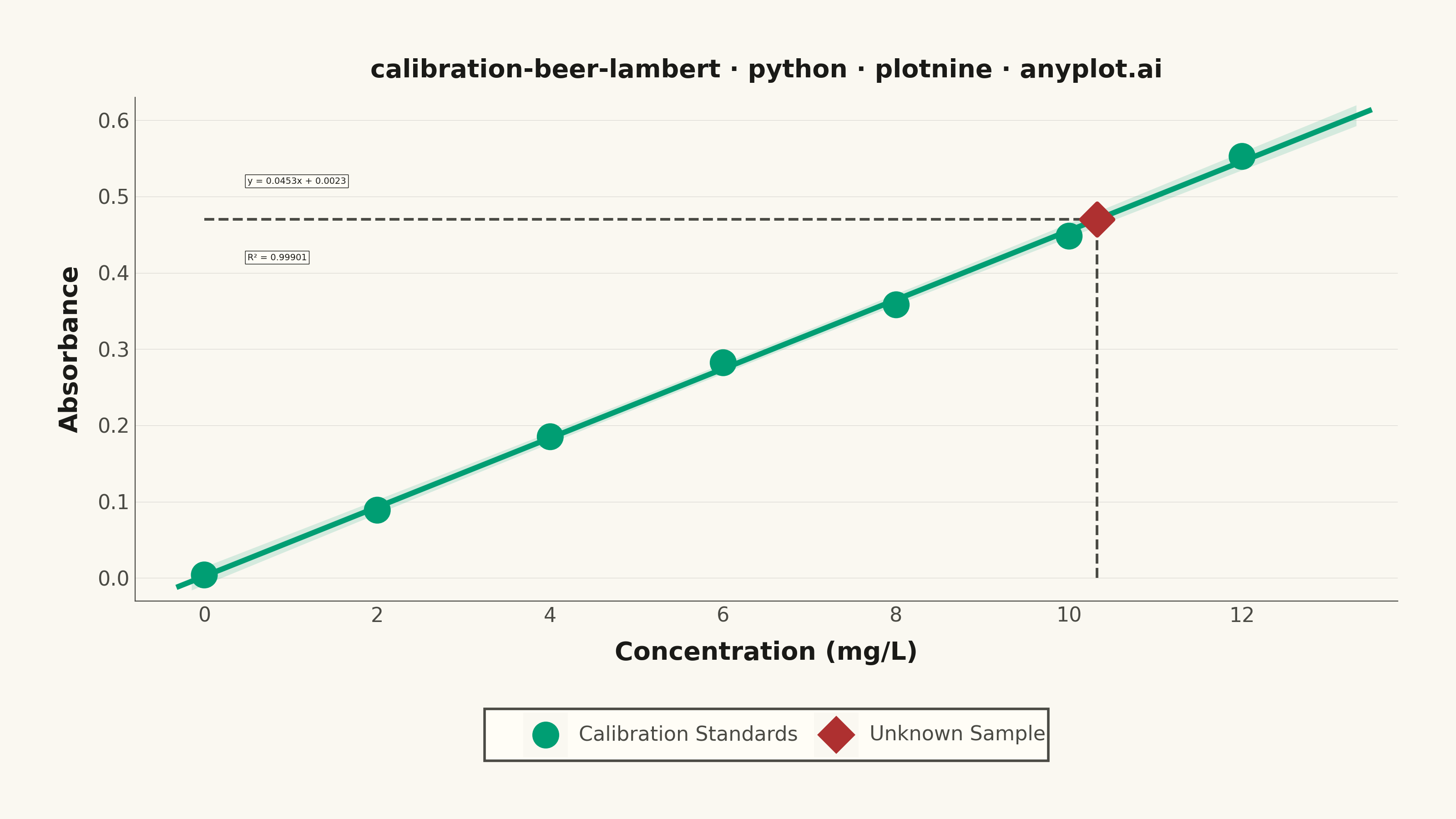
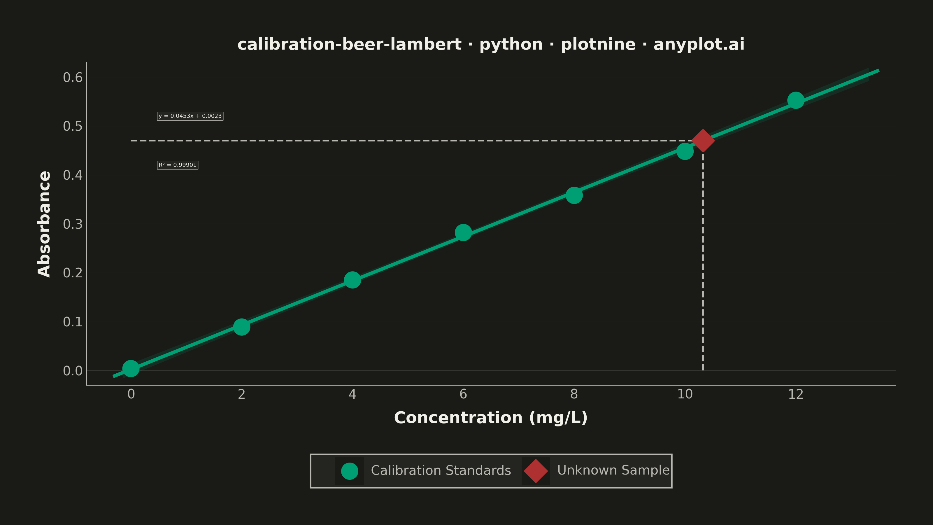
A calibration curve plotting absorbance versus concentration following Beer-Lambert law (A = εlc). Measured calibration standards are shown as scatter points with a linear regression fit line. The regression equation (y = mx + b) and R² value are displayed on the plot. An example unknown sample is marked with dashed lines extending to both axes, demonstrating how the curve is used to determine concentration from a measured absorbance. This plot is fundamental in analytical chemistry for quantitative spectrophotometric analysis.
""" anyplot.ai
calibration-beer-lambert: Beer-Lambert Calibration Curve
Library: plotnine 0.15.5 | Python 3.13.13
Quality: 89/100 | Updated: 2026-06-03
"""

import os

import numpy as np
import pandas as pd
from plotnine import (
    aes,
    element_blank,
    element_line,
    element_rect,
    element_text,
    geom_label,
    geom_point,
    geom_segment,
    ggplot,
    labs,
    scale_color_manual,
    scale_fill_manual,
    scale_shape_manual,
    scale_x_continuous,
    scale_y_continuous,
    stat_smooth,
    theme,
    theme_minimal,
)
from scipy import stats


# Theme tokens — Imprint palette, theme-adaptive chrome
THEME = os.getenv("ANYPLOT_THEME", "light")
PAGE_BG = "#FAF8F1" if THEME == "light" else "#1A1A17"
ELEVATED_BG = "#FFFDF6" if THEME == "light" else "#242420"
INK = "#1A1A17" if THEME == "light" else "#F0EFE8"
INK_SOFT = "#4A4A44" if THEME == "light" else "#B8B7B0"

# Imprint palette — positions 1 and 5 (green = calibration standards, red = unknown)
BRAND = "#009E73"  # position 1 — always first series
UNKNOWN_COLOR = "#AE3030"  # position 5 — semantic red for "unknown" highlight

# Data
np.random.seed(42)
concentrations = np.array([0.0, 2.0, 4.0, 6.0, 8.0, 10.0, 12.0])
molar_absorptivity = 0.045
absorbances = molar_absorptivity * concentrations + np.random.normal(0, 0.008, len(concentrations))
absorbances = np.clip(absorbances, 0, None)

# Linear regression
slope, intercept, r_value, p_value, std_err = stats.linregress(concentrations, absorbances)
r_squared = r_value**2

# Unknown sample — ~10.5 mg/L (differentiated from Letsplot sibling at 7.5 mg/L)
unknown_absorbance = 0.47
unknown_concentration = (unknown_absorbance - intercept) / slope

df_standards = pd.DataFrame(
    {"concentration": concentrations, "absorbance": absorbances, "series": "Calibration Standards"}
)

df_unknown = pd.DataFrame(
    {"concentration": [unknown_concentration], "absorbance": [unknown_absorbance], "series": "Unknown Sample"}
)

df_all = pd.concat([df_standards, df_unknown], ignore_index=True)

# Dashed projection lines to both axes
df_seg_h = pd.DataFrame(
    {"x": [0.0], "xend": [unknown_concentration], "y": [unknown_absorbance], "yend": [unknown_absorbance]}
)
df_seg_v = pd.DataFrame(
    {"x": [unknown_concentration], "xend": [unknown_concentration], "y": [0.0], "yend": [unknown_absorbance]}
)

# Annotation text
eq_text = f"y = {slope:.4f}x + {intercept:.4f}"
r2_text = f"R² = {r_squared:.5f}"

df_eq = pd.DataFrame({"x": [0.5], "y": [0.52], "label": [eq_text]})
df_r2 = pd.DataFrame({"x": [0.5], "y": [0.42], "label": [r2_text]})

# Plot
plot = (
    ggplot(df_standards, aes(x="concentration", y="absorbance"))
    + stat_smooth(method="lm", color=BRAND, fill=BRAND, alpha=0.15, size=1.2, fullrange=True)
    + geom_segment(
        df_seg_h,
        aes(x="x", xend="xend", y="y", yend="yend"),
        linetype="dashed",
        color=INK_SOFT,
        size=0.6,
        inherit_aes=False,
    )
    + geom_segment(
        df_seg_v,
        aes(x="x", xend="xend", y="y", yend="yend"),
        linetype="dashed",
        color=INK_SOFT,
        size=0.6,
        inherit_aes=False,
    )
    + geom_point(
        df_all,
        aes(x="concentration", y="absorbance", color="series", shape="series", fill="series"),
        size=4,
        stroke=1.0,
        inherit_aes=False,
    )
    + scale_color_manual(values={"Calibration Standards": BRAND, "Unknown Sample": UNKNOWN_COLOR}, name=" ")
    + scale_fill_manual(values={"Calibration Standards": BRAND, "Unknown Sample": UNKNOWN_COLOR}, name=" ")
    + scale_shape_manual(values={"Calibration Standards": "o", "Unknown Sample": "D"}, name=" ")
    + geom_label(
        df_eq,
        aes(x="x", y="y", label="label"),
        ha="left",
        size=3.5,
        color=INK,
        fill=ELEVATED_BG,
        label_size=0.25,
        label_r=0.03,
        inherit_aes=False,
        show_legend=False,
    )
    + geom_label(
        df_r2,
        aes(x="x", y="y", label="label"),
        ha="left",
        size=3.5,
        color=INK,
        fill=ELEVATED_BG,
        label_size=0.25,
        label_r=0.03,
        inherit_aes=False,
        show_legend=False,
    )
    + scale_x_continuous(breaks=np.arange(0, 14, 2), limits=(-0.5, 13.5), expand=(0, 0.3))
    + scale_y_continuous(breaks=np.arange(0, 0.65, 0.1), limits=(-0.02, 0.62), expand=(0, 0.01))
    + labs(x="Concentration (mg/L)", y="Absorbance", title="calibration-beer-lambert · python · plotnine · anyplot.ai")
    + theme_minimal()
    + theme(
        figure_size=(8, 4.5),
        text=element_text(size=7, family="sans-serif"),
        axis_title=element_text(size=10, weight="bold", color=INK),
        axis_text=element_text(size=8, color=INK_SOFT),
        plot_title=element_text(size=10, weight="bold", color=INK),
        plot_background=element_rect(fill=PAGE_BG, color=PAGE_BG),
        panel_background=element_rect(fill=PAGE_BG),
        panel_grid_major_x=element_blank(),
        panel_grid_minor=element_blank(),
        panel_grid_major_y=element_line(color=INK, size=0.2, alpha=0.15),
        axis_line_x=element_line(color=INK_SOFT, size=0.4),
        axis_line_y=element_line(color=INK_SOFT, size=0.4),
        legend_position="bottom",
        legend_text=element_text(size=8, color=INK_SOFT),
        legend_title=element_text(color=INK),
        legend_background=element_rect(fill=ELEVATED_BG, color=INK_SOFT),
        legend_key=element_rect(fill=PAGE_BG, color=PAGE_BG),
        plot_margin=0.04,
    )
)

# Save — canonical 3200×1800 px (8 in × 4.5 in @ dpi=400)
plot.save(f"plot-{THEME}.png", dpi=400, width=8, height=4.5, units="in", verbose=False)
Runnable source as JSON, for any HTTP client: https://api.anyplot.ai/specs/calibration-beer-lambert/plotnine/code. Any spec id and library id listed in llms-full.txt fit the same URL shape; every URL below is complete and callable.
{
  "spec_id": "calibration-beer-lambert",
  "language": "python",
  "library": "plotnine",
  "page": "https://anyplot.ai/calibration-beer-lambert/python/plotnine",
  "hub": "https://anyplot.ai/calibration-beer-lambert",
  "code_json": "https://api.anyplot.ai/specs/calibration-beer-lambert/plotnine/code",
  "spec_json": "https://api.anyplot.ai/specs/calibration-beer-lambert",
  "render_light_png": "https://storage.googleapis.com/anyplot-images/plots/calibration-beer-lambert/python/plotnine/plot-light.png",
  "render_dark_png": "https://storage.googleapis.com/anyplot-images/plots/calibration-beer-lambert/python/plotnine/plot-dark.png",
  "quality_score": 89.0,
  "license": "MIT",
  "guide": "https://anyplot.ai/llms.txt"
}
Part of Beer-Lambert Calibration Curve on anyplot.ai.