The same plot in 14 other libraries — JavaScript: Chart.js, D3.js, Apache ECharts, MUI X Charts; Python: Altair, Bokeh, lets-plot, Matplotlib, Plotly, plotnine, Pygal, Seaborn; R: ggplot2; Julia: Makie.jl. Compare all 15 side by side: Beer-Lambert Calibration Curve in Python, R, Julia and JavaScript.
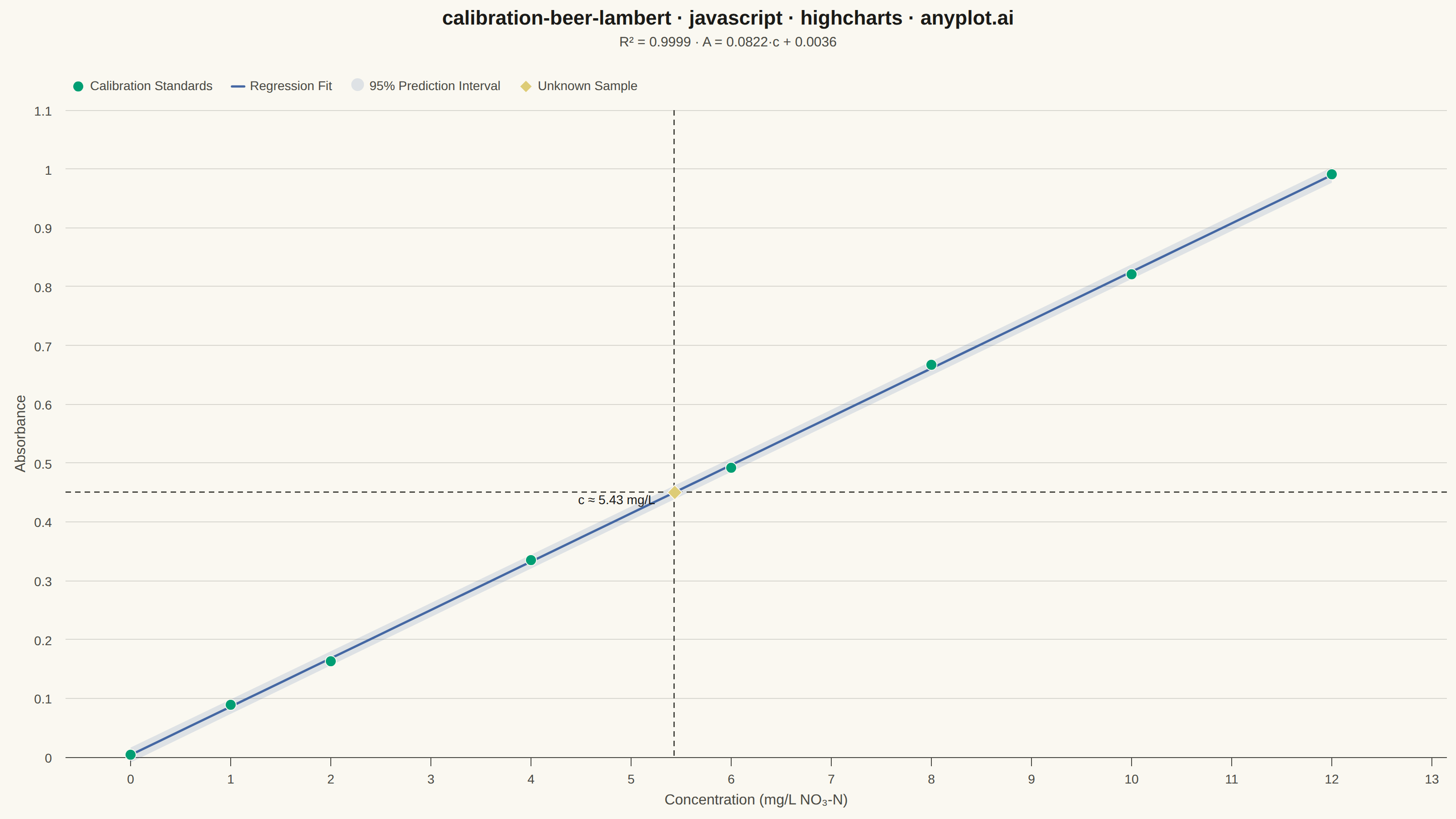
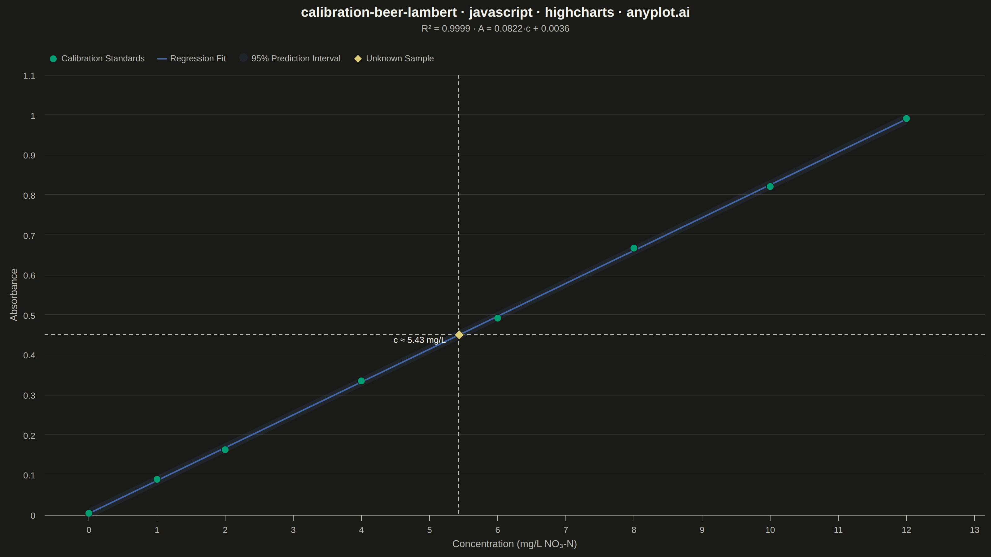
A calibration curve plotting absorbance versus concentration following Beer-Lambert law (A = εlc). Measured calibration standards are shown as scatter points with a linear regression fit line. The regression equation (y = mx + b) and R² value are displayed on the plot. An example unknown sample is marked with dashed lines extending to both axes, demonstrating how the curve is used to determine concentration from a measured absorbance. This plot is fundamental in analytical chemistry for quantitative spectrophotometric analysis.
// anyplot.ai
// calibration-beer-lambert: Beer-Lambert Calibration Curve
// Library: highcharts 12.6.0 | JavaScript 22.23.2
// Quality: 92/100 | Created: 2026-08-20

const t = window.ANYPLOT_TOKENS;

// --- Data: nitrate colorimetric assay standards, 540 nm ---------------------
// concentration in mg/L NO3-N, absorbance dimensionless (incl. reagent blank)
const standards = [
  [0, 0.004],
  [1, 0.089],
  [2, 0.163],
  [4, 0.335],
  [6, 0.492],
  [8, 0.667],
  [10, 0.821],
  [12, 0.991],
];
const n = standards.length;

// --- Ordinary least-squares fit ---------------------------------------------
const xs = standards.map((p) => p[0]);
const ys = standards.map((p) => p[1]);
const xBar = xs.reduce((a, b) => a + b, 0) / n;
const yBar = ys.reduce((a, b) => a + b, 0) / n;
let sxx = 0;
let sxy = 0;
let syy = 0;
for (let i = 0; i < n; i++) {
  const dx = xs[i] - xBar;
  const dy = ys[i] - yBar;
  sxx += dx * dx;
  sxy += dx * dy;
  syy += dy * dy;
}
const slope = sxy / sxx;
const intercept = yBar - slope * xBar;
const r2 = (sxy * sxy) / (sxx * syy);
const sse = ys.reduce((acc, y, i) => acc + (y - (slope * xs[i] + intercept)) ** 2, 0);
const residualStdErr = Math.sqrt(sse / (n - 2));
const tCrit = 2.447; // 95% two-tail critical value at df=6

// Regression line + 95% prediction interval band across the standards' range.
const xMin = Math.min(...xs);
const xMax = Math.max(...xs);
const steps = 40;
const lineData = [];
const piUpper = [];
const piLower = [];
for (let i = 0; i <= steps; i++) {
  const x0 = xMin + ((xMax - xMin) * i) / steps;
  const yHat = slope * x0 + intercept;
  const se = residualStdErr * Math.sqrt(1 + 1 / n + (x0 - xBar) ** 2 / sxx);
  lineData.push([x0, yHat]);
  piUpper.push([x0, yHat + tCrit * se]);
  piLower.push([x0, yHat - tCrit * se]);
}

// Example unknown sample: measured absorbance, back-calculated concentration.
const unknownAbsorbance = 0.45;
const unknownConcentration = (unknownAbsorbance - intercept) / slope;

// --- Chart -------------------------------------------------------------------
// arearange lives in highcharts-more (not vendored), so the prediction band is
// drawn as a plain SVG path in the core renderer, redrawn on every chart render.
let bandPath;
Highcharts.chart("container", {
  chart: {
    type: "scatter",
    backgroundColor: "transparent",
    animation: false,
    style: { fontFamily: "inherit" },
    events: {
      render: function () {
        const xAxis = this.xAxis[0];
        const yAxis = this.yAxis[0];
        const upper = piUpper.map(
          (p, i) => `${i === 0 ? "M" : "L"} ${xAxis.toPixels(p[0], false)} ${yAxis.toPixels(p[1], false)}`,
        );
        const lower = piLower
          .slice()
          .reverse()
          .map((p) => `L ${xAxis.toPixels(p[0], false)} ${yAxis.toPixels(p[1], false)}`);
        const d = `${upper.join(" ")} ${lower.join(" ")} Z`;
        if (bandPath) {
          bandPath.attr({ d });
        } else {
          bandPath = this.renderer
            .path()
            .attr({ d, fill: Highcharts.color(t.palette[2]).setOpacity(0.15).get(), zIndex: 2 })
            .add();
        }
      },
    },
  },
  credits: { enabled: false },
  colors: t.palette,
  title: {
    text: "calibration-beer-lambert · javascript · highcharts · anyplot.ai",
    style: { color: t.ink, fontSize: "22px", fontWeight: "600" },
  },
  subtitle: {
    text: `R² = ${r2.toFixed(4)}  ·  A = ${slope.toFixed(4)}·c + ${intercept.toFixed(4)}`,
    style: { color: t.inkSoft, fontSize: "15px" },
  },
  xAxis: {
    title: { text: "Concentration (mg/L NO₃-N)", style: { color: t.inkSoft, fontSize: "16px" } },
    lineColor: t.inkSoft,
    tickColor: t.inkSoft,
    gridLineColor: t.grid,
    labels: { style: { color: t.inkSoft, fontSize: "14px" } },
    min: -0.5,
    max: xMax + 1,
    plotLines: [
      {
        value: unknownConcentration,
        color: t.inkSoft,
        dashStyle: "Dash",
        width: 1.5,
        zIndex: 3,
      },
    ],
  },
  yAxis: {
    title: { text: "Absorbance", style: { color: t.inkSoft, fontSize: "16px" } },
    lineColor: t.inkSoft,
    tickColor: t.inkSoft,
    gridLineColor: t.grid,
    labels: { style: { color: t.inkSoft, fontSize: "14px" } },
    min: 0,
    plotLines: [
      {
        value: unknownAbsorbance,
        color: t.inkSoft,
        dashStyle: "Dash",
        width: 1.5,
        zIndex: 3,
      },
    ],
  },
  legend: {
    align: "left",
    verticalAlign: "top",
    x: 60,
    y: 10,
    itemStyle: { color: t.inkSoft, fontSize: "14px" },
    itemHoverStyle: { color: t.ink },
  },
  tooltip: {
    pointFormat: "Concentration: {point.x:.2f} mg/L<br/>Absorbance: {point.y:.3f}",
  },
  plotOptions: {
    series: { animation: false },
  },
  series: [
    {
      type: "scatter",
      name: "Calibration Standards",
      data: standards,
      zIndex: 5,
      marker: {
        radius: 6,
        fillColor: t.palette[0],
        lineColor: t.pageBg,
        lineWidth: 1,
      },
    },
    {
      type: "line",
      name: "Regression Fit",
      data: lineData,
      color: t.palette[2],
      lineWidth: 2.5,
      zIndex: 4,
      marker: { enabled: false },
      enableMouseTracking: false,
    },
    {
      type: "column",
      name: "95% Prediction Interval",
      data: [],
      color: Highcharts.color(t.palette[2]).setOpacity(0.15).get(),
      legendSymbol: "rectangle",
      showInLegend: true,
      enableMouseTracking: false,
    },
    {
      type: "scatter",
      name: "Unknown Sample",
      data: [{ x: unknownConcentration, y: unknownAbsorbance }],
      zIndex: 6,
      marker: {
        symbol: "diamond",
        radius: 8,
        fillColor: t.amber,
        lineColor: t.pageBg,
        lineWidth: 1,
      },
      dataLabels: {
        enabled: true,
        format: `c ≈ ${unknownConcentration.toFixed(2)} mg/L`,
        style: { color: t.ink, fontSize: "14px", fontWeight: "500", textOutline: "none" },
        align: "right",
        x: -16,
        y: 20,
      },
    },
  ],
});
Runnable source as JSON, for any HTTP client: https://api.anyplot.ai/specs/calibration-beer-lambert/highcharts/code. Any spec id and library id listed in llms-full.txt fit the same URL shape; every URL below is complete and callable.
{
  "spec_id": "calibration-beer-lambert",
  "language": "javascript",
  "library": "highcharts",
  "page": "https://anyplot.ai/calibration-beer-lambert/javascript/highcharts",
  "hub": "https://anyplot.ai/calibration-beer-lambert",
  "code_json": "https://api.anyplot.ai/specs/calibration-beer-lambert/highcharts/code",
  "spec_json": "https://api.anyplot.ai/specs/calibration-beer-lambert",
  "render_light_png": "https://storage.googleapis.com/anyplot-images/plots/calibration-beer-lambert/javascript/highcharts/plot-light.png",
  "render_dark_png": "https://storage.googleapis.com/anyplot-images/plots/calibration-beer-lambert/javascript/highcharts/plot-dark.png",
  "interactive_light_html": "https://storage.googleapis.com/anyplot-images/plots/calibration-beer-lambert/javascript/highcharts/plot-light.html",
  "interactive_dark_html": "https://storage.googleapis.com/anyplot-images/plots/calibration-beer-lambert/javascript/highcharts/plot-dark.html",
  "quality_score": 92.0,
  "license": "MIT",
  "guide": "https://anyplot.ai/llms.txt"
}
Part of Beer-Lambert Calibration Curve on anyplot.ai.