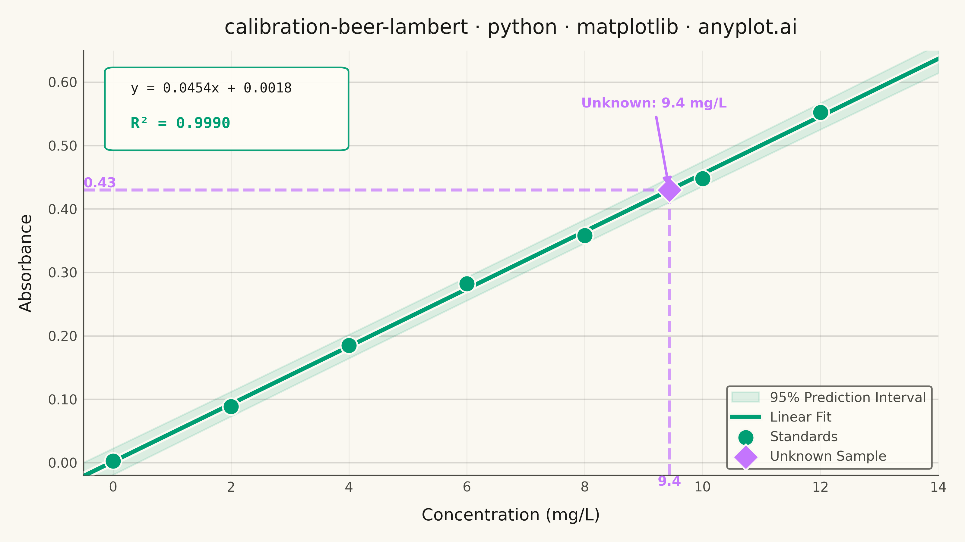
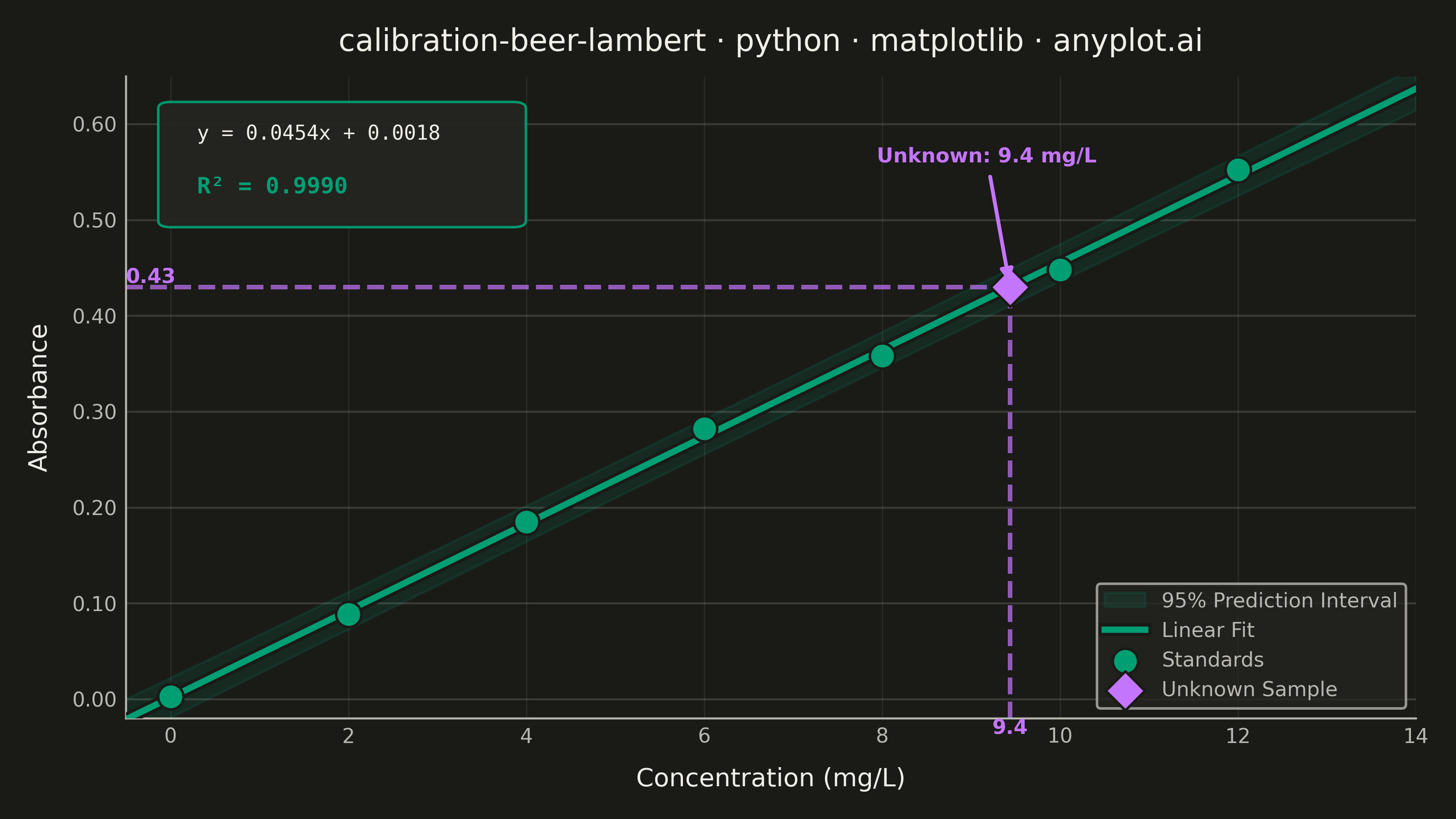
A calibration curve plotting absorbance versus concentration following Beer-Lambert law (A = εlc). Measured calibration standards are shown as scatter points with a linear regression fit line. The regression equation (y = mx + b) and R² value are displayed on the plot. An example unknown sample is marked with dashed lines extending to both axes, demonstrating how the curve is used to determine concentration from a measured absorbance. This plot is fundamental in analytical chemistry for quantitative spectrophotometric analysis.
""" anyplot.ai
calibration-beer-lambert: Beer-Lambert Calibration Curve
Library: matplotlib 3.10.9 | Python 3.13.13
Quality: 90/100 | Updated: 2026-06-03
"""

import os

import matplotlib.patheffects as pe
import matplotlib.pyplot as plt
import matplotlib.ticker as ticker
import numpy as np
from matplotlib.patches import FancyBboxPatch
from scipy import stats


# Theme tokens
THEME = os.getenv("ANYPLOT_THEME", "light")
PAGE_BG = "#FAF8F1" if THEME == "light" else "#1A1A17"
ELEVATED_BG = "#FFFDF6" if THEME == "light" else "#242420"
INK = "#1A1A17" if THEME == "light" else "#F0EFE8"
INK_SOFT = "#4A4A44" if THEME == "light" else "#B8B7B0"
INK_MUTED = "#6B6A63" if THEME == "light" else "#A8A79F"

# Imprint palette positions 1 and 2
STANDARDS_COLOR = "#009E73"  # position 1 — calibration standards and fit
UNKNOWN_COLOR = "#C475FD"  # position 2 — unknown sample

# Data
np.random.seed(42)
concentrations = np.array([0.0, 2.0, 4.0, 6.0, 8.0, 10.0, 12.0])
molar_absorptivity = 0.045
absorbances = molar_absorptivity * concentrations + np.random.normal(0, 0.008, len(concentrations))
absorbances[0] = 0.003

# Linear regression
slope, intercept, r_value, p_value, std_err = stats.linregress(concentrations, absorbances)
r_squared = r_value**2

# Regression line and 95% prediction interval
conc_fit = np.linspace(-0.5, 14, 200)
abs_fit = slope * conc_fit + intercept

n = len(concentrations)
conc_mean = np.mean(concentrations)
residual_std = np.sqrt(np.sum((absorbances - slope * concentrations - intercept) ** 2) / (n - 2))
se_pred = residual_std * np.sqrt(1 + 1 / n + (conc_fit - conc_mean) ** 2 / np.sum((concentrations - conc_mean) ** 2))
t_crit = stats.t.ppf(0.975, n - 2)
pred_upper = abs_fit + t_crit * se_pred
pred_lower = abs_fit - t_crit * se_pred

# Unknown sample at ~9.5 mg/L (distinct from sibling implementations)
unknown_absorbance = 0.43
unknown_concentration = (unknown_absorbance - intercept) / slope

# Plot — 3200×1800 px landscape canvas
fig, ax = plt.subplots(figsize=(8, 4.5), dpi=400, facecolor=PAGE_BG)
ax.set_facecolor(PAGE_BG)

# Prediction interval band
ax.fill_between(
    conc_fit, pred_lower, pred_upper, alpha=0.12, color=STANDARDS_COLOR, label="95% Prediction Interval", zorder=1
)

# Fit line — PathEffects halo makes it pop above overlapping markers
(fit_line,) = ax.plot(conc_fit, abs_fit, color=STANDARDS_COLOR, linewidth=2.5, zorder=3, label="Linear Fit")
fit_line.set_path_effects([pe.withStroke(linewidth=5, foreground=PAGE_BG)])

# Calibration standards
ax.scatter(
    concentrations,
    absorbances,
    s=100,
    color=STANDARDS_COLOR,
    edgecolors=PAGE_BG,
    linewidth=1.0,
    zorder=5,
    label="Standards",
)

# Unknown sample dashed guide lines
ax.plot(
    [unknown_concentration, unknown_concentration],
    [-0.02, unknown_absorbance],
    linestyle="--",
    color=UNKNOWN_COLOR,
    linewidth=1.8,
    alpha=0.7,
    zorder=2,
)
ax.plot(
    [-0.5, unknown_concentration],
    [unknown_absorbance, unknown_absorbance],
    linestyle="--",
    color=UNKNOWN_COLOR,
    linewidth=1.8,
    alpha=0.7,
    zorder=2,
)

# Unknown sample marker
ax.scatter(
    [unknown_concentration],
    [unknown_absorbance],
    s=120,
    color=UNKNOWN_COLOR,
    edgecolors=PAGE_BG,
    linewidth=1.0,
    zorder=6,
    marker="D",
    label="Unknown Sample",
)

# Regression equation annotation — FancyBboxPatch background + two text elements
# for visual hierarchy: R² line rendered bold in brand green
ann_patch = FancyBboxPatch(
    (0.035, 0.775),
    0.265,
    0.175,
    boxstyle="round,pad=0.01",
    transform=ax.transAxes,
    facecolor=ELEVATED_BG,
    edgecolor=STANDARDS_COLOR,
    alpha=0.95,
    linewidth=1.0,
    zorder=7,
)
ax.add_patch(ann_patch)
ax.text(
    0.055,
    0.925,
    f"y = {slope:.4f}x + {intercept:.4f}",
    transform=ax.transAxes,
    fontsize=8,
    fontfamily="monospace",
    verticalalignment="top",
    color=INK,
    zorder=8,
)
ax.text(
    0.055,
    0.845,
    f"R² = {r_squared:.4f}",
    transform=ax.transAxes,
    fontsize=9,
    fontfamily="monospace",
    fontweight="bold",
    verticalalignment="top",
    color=STANDARDS_COLOR,
    zorder=8,
)

# Unknown annotation with arrow
ax.annotate(
    f"Unknown: {unknown_concentration:.1f} mg/L",
    xy=(unknown_concentration, unknown_absorbance),
    xytext=(unknown_concentration - 1.5, unknown_absorbance + 0.13),
    fontsize=8,
    fontweight="semibold",
    color=UNKNOWN_COLOR,
    arrowprops={"arrowstyle": "-|>", "color": UNKNOWN_COLOR, "lw": 1.5, "mutation_scale": 10},
    zorder=7,
)

# Axis value markers at the unknown's intercept points
ax.annotate(
    f"{unknown_concentration:.1f}",
    xy=(unknown_concentration, -0.02),
    fontsize=8,
    color=UNKNOWN_COLOR,
    fontweight="bold",
    ha="center",
    va="top",
)
ax.annotate(
    f"{unknown_absorbance:.2f}",
    xy=(-0.5, unknown_absorbance),
    fontsize=8,
    color=UNKNOWN_COLOR,
    fontweight="bold",
    ha="left",
    va="bottom",
)

# Style
title = "calibration-beer-lambert · python · matplotlib · anyplot.ai"
title_fontsize = max(8, round(12 * 67 / len(title))) if len(title) > 67 else 12
ax.set_title(title, fontsize=title_fontsize, fontweight="medium", pad=10, color=INK)
ax.set_xlabel("Concentration (mg/L)", fontsize=10, labelpad=8, color=INK)
ax.set_ylabel("Absorbance", fontsize=10, labelpad=8, color=INK)
ax.tick_params(axis="both", labelsize=8, colors=INK_SOFT, labelcolor=INK_SOFT, length=0)
for spine in ["top", "right"]:
    ax.spines[spine].set_visible(False)
for spine in ["bottom", "left"]:
    ax.spines[spine].set_color(INK_SOFT)

# Custom absorbance formatter — two decimal places on y-axis ticks
ax.yaxis.set_major_formatter(ticker.FormatStrFormatter("%.2f"))

ax.yaxis.grid(True, alpha=0.15, linewidth=0.8, color=INK)
ax.xaxis.grid(True, alpha=0.08, linewidth=0.5, color=INK)
ax.set_xlim(-0.5, 14)
ax.set_ylim(-0.02, 0.65)

leg = ax.legend(fontsize=8, loc="lower right")
if leg:
    leg.get_frame().set_facecolor(ELEVATED_BG)
    leg.get_frame().set_edgecolor(INK_SOFT)
    plt.setp(leg.get_texts(), color=INK_SOFT)

plt.tight_layout()
plt.savefig(f"plot-{THEME}.png", dpi=400, facecolor=PAGE_BG)
Runnable source as JSON, for any HTTP client: https://api.anyplot.ai/specs/calibration-beer-lambert/matplotlib/code. Any spec id and library id listed in llms-full.txt fit the same URL shape; every URL below is complete and callable.
{
  "spec_id": "calibration-beer-lambert",
  "language": "python",
  "library": "matplotlib",
  "page": "https://anyplot.ai/calibration-beer-lambert/python/matplotlib",
  "hub": "https://anyplot.ai/calibration-beer-lambert",
  "code_json": "https://api.anyplot.ai/specs/calibration-beer-lambert/matplotlib/code",
  "spec_json": "https://api.anyplot.ai/specs/calibration-beer-lambert",
  "render_light_png": "https://storage.googleapis.com/anyplot-images/plots/calibration-beer-lambert/python/matplotlib/plot-light.png",
  "render_dark_png": "https://storage.googleapis.com/anyplot-images/plots/calibration-beer-lambert/python/matplotlib/plot-dark.png",
  "quality_score": 90.0,
  "license": "MIT",
  "guide": "https://anyplot.ai/llms.txt"
}
Part of Beer-Lambert Calibration Curve on anyplot.ai.