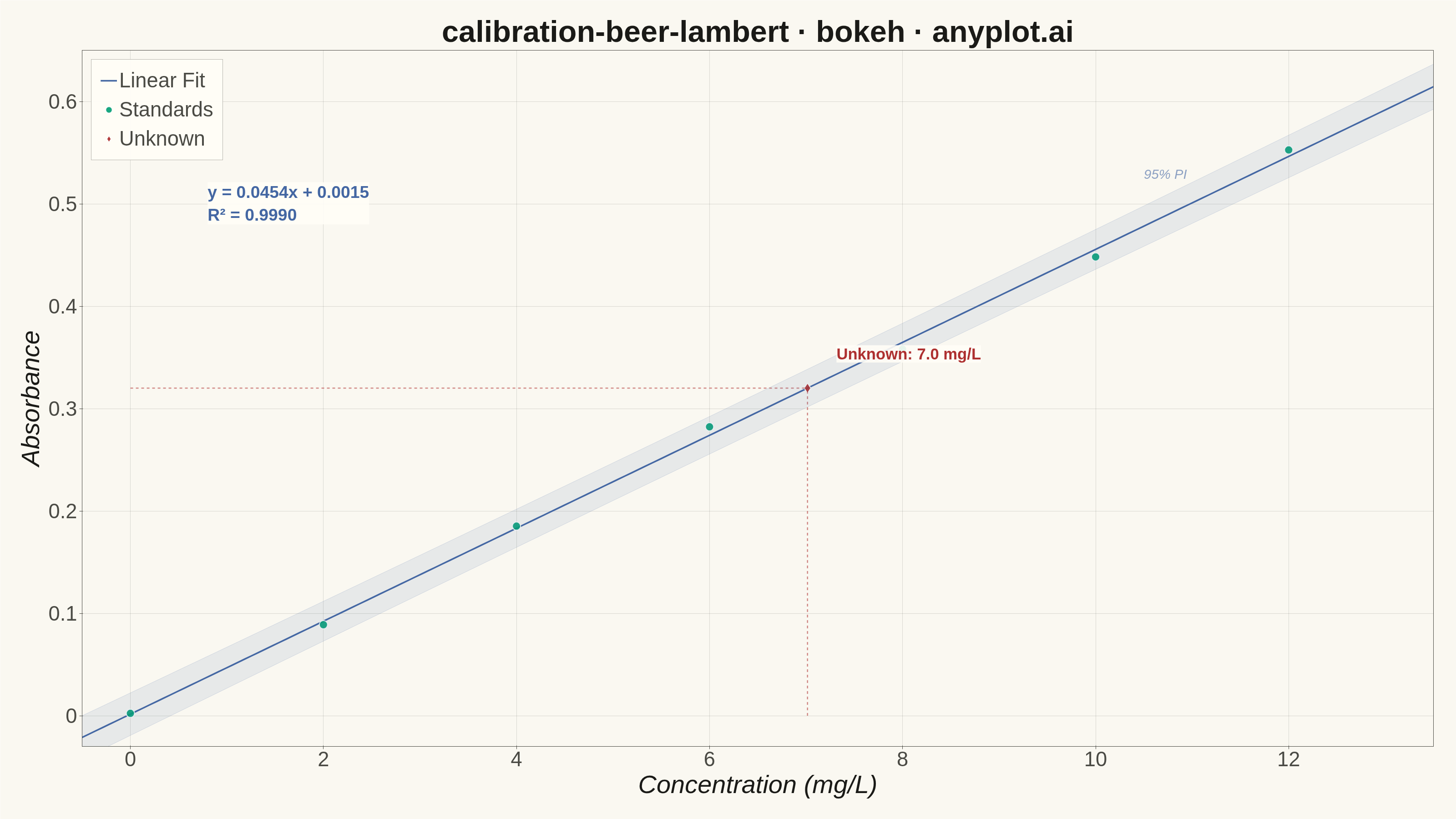
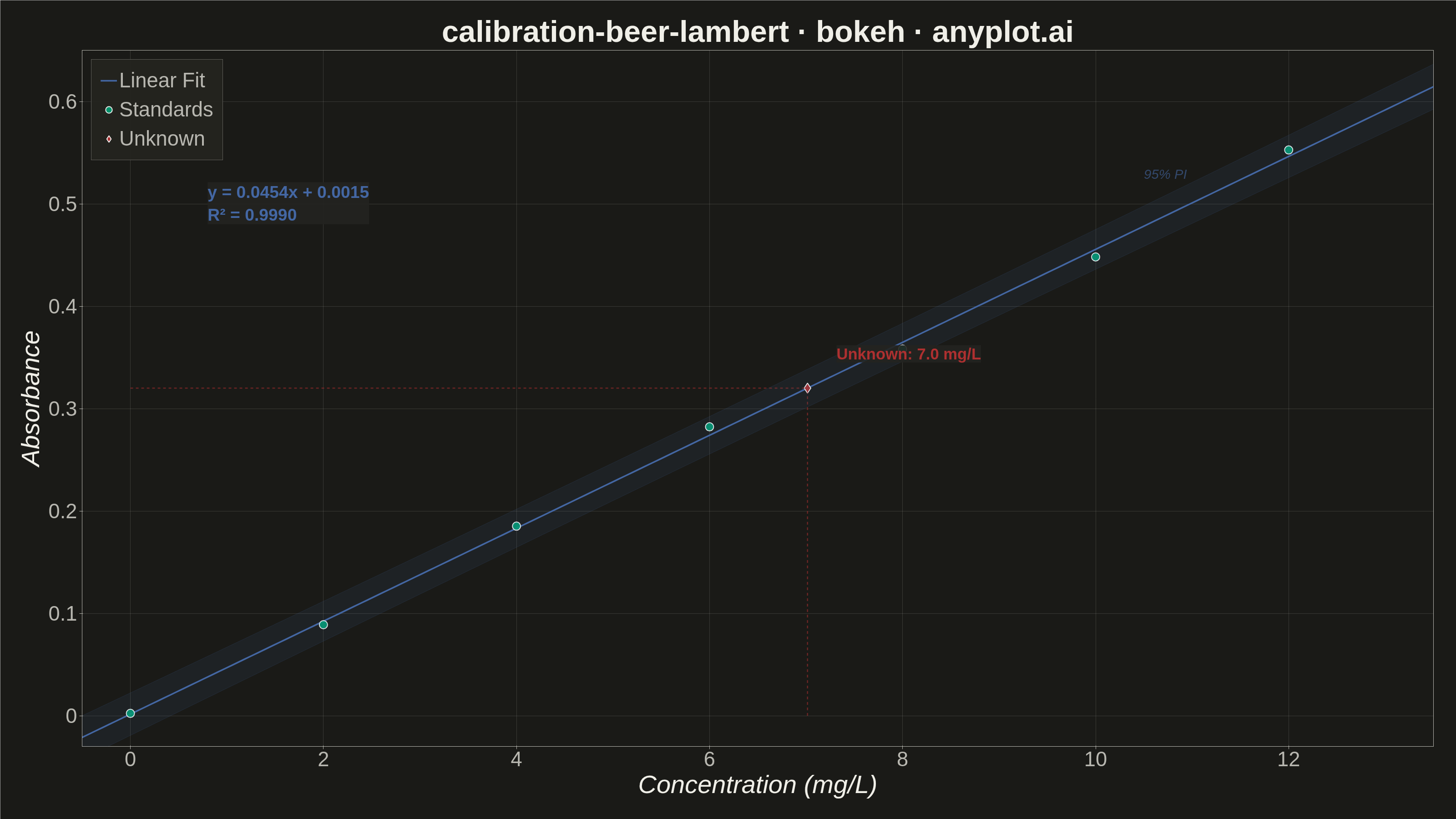
A calibration curve plotting absorbance versus concentration following Beer-Lambert law (A = εlc). Measured calibration standards are shown as scatter points with a linear regression fit line. The regression equation (y = mx + b) and R² value are displayed on the plot. An example unknown sample is marked with dashed lines extending to both axes, demonstrating how the curve is used to determine concentration from a measured absorbance. This plot is fundamental in analytical chemistry for quantitative spectrophotometric analysis.
""" anyplot.ai
calibration-beer-lambert: Beer-Lambert Calibration Curve
Library: bokeh 3.9.0 | Python 3.13.13
Quality: 90/100 | Updated: 2026-06-03
"""

import os
import time
from pathlib import Path

import numpy as np
from bokeh.io import output_file, save
from bokeh.models import Band, ColumnDataSource, HoverTool, Label
from bokeh.plotting import figure
from PIL import Image as _PILImage
from scipy import stats
from selenium import webdriver
from selenium.webdriver.chrome.options import Options


THEME = os.getenv("ANYPLOT_THEME", "light")

# Imprint palette — theme-independent
IMPRINT_PALETTE = ["#009E73", "#C475FD", "#4467A3", "#BD8233", "#AE3030", "#2ABCCD", "#954477", "#99B314"]
BRAND = IMPRINT_PALETTE[0]  # #009E73 — always first series

# Theme-adaptive chrome tokens
PAGE_BG = "#FAF8F1" if THEME == "light" else "#1A1A17"
ELEVATED_BG = "#FFFDF6" if THEME == "light" else "#242420"
INK = "#1A1A17" if THEME == "light" else "#F0EFE8"
INK_SOFT = "#4A4A44" if THEME == "light" else "#B8B7B0"
INK_MUTED = "#6B6A63" if THEME == "light" else "#A8A79F"

# Semantic colors for this chart
STANDARDS_COLOR = BRAND  # #009E73 — Imprint position 1
FIT_COLOR = IMPRINT_PALETTE[2]  # #4467A3 — blue for the regression line
UNKNOWN_COLOR = IMPRINT_PALETTE[4]  # #AE3030 — semantic red for unknown sample

# Data — UV-Vis calibration standards for copper sulfate at 810 nm
np.random.seed(42)
concentrations = np.array([0.0, 2.0, 4.0, 6.0, 8.0, 10.0, 12.0])
epsilon_l = 0.045  # molar absorptivity × path length
true_absorbance = epsilon_l * concentrations
noise = np.random.normal(0, 0.008, len(concentrations))
noise[0] = np.random.normal(0, 0.003)  # blank has less noise
absorbance = true_absorbance + noise
absorbance[0] = max(0.001, absorbance[0])

# Linear regression
slope, intercept, r_value, p_value, std_err = stats.linregress(concentrations, absorbance)
r_squared = r_value**2

# Regression line and 95% prediction interval
conc_line = np.linspace(-0.5, 13.5, 200)
abs_line = slope * conc_line + intercept

n = len(concentrations)
conc_mean = np.mean(concentrations)
residuals = absorbance - (slope * concentrations + intercept)
se = np.sqrt(np.sum(residuals**2) / (n - 2))
t_val = stats.t.ppf(0.975, n - 2)

se_pred = se * np.sqrt(1 + 1 / n + (conc_line - conc_mean) ** 2 / np.sum((concentrations - conc_mean) ** 2))
pi_upper = abs_line + t_val * se_pred
pi_lower = abs_line - t_val * se_pred

# Unknown sample back-calculated concentration
unknown_absorbance = 0.32
unknown_concentration = (unknown_absorbance - intercept) / slope

# ColumnDataSources
scatter_source = ColumnDataSource(
    data={
        "conc": concentrations,
        "abs": absorbance,
        "conc_fmt": [f"{c:.1f}" for c in concentrations],
        "abs_fmt": [f"{a:.4f}" for a in absorbance],
    }
)
line_source = ColumnDataSource(data={"conc": conc_line, "abs": abs_line})
band_source = ColumnDataSource(data={"conc": conc_line, "lower": pi_lower, "upper": pi_upper})
unknown_source = ColumnDataSource(
    data={
        "conc": [unknown_concentration],
        "abs": [unknown_absorbance],
        "conc_fmt": [f"{unknown_concentration:.2f}"],
        "abs_fmt": [f"{unknown_absorbance:.4f}"],
    }
)

# Figure — 3200×1800 landscape with toolbar disabled for PNG accuracy
p = figure(
    width=3200,
    height=1800,
    title="calibration-beer-lambert · bokeh · anyplot.ai",
    x_axis_label="Concentration (mg/L)",
    y_axis_label="Absorbance",
    x_range=(-0.5, 13.5),
    y_range=(-0.03, 0.65),
    toolbar_location=None,  # prevents the toolbar from adding ~30–50 px above the canvas
    min_border_bottom=160,
    min_border_left=180,
    min_border_top=110,
    min_border_right=50,
)

# Backgrounds
p.background_fill_color = PAGE_BG
p.border_fill_color = PAGE_BG
p.outline_line_color = INK_SOFT

# 95% prediction interval band
band = Band(
    base="conc",
    lower="lower",
    upper="upper",
    source=band_source,
    fill_color=FIT_COLOR,
    fill_alpha=0.10,
    line_color=FIT_COLOR,
    line_alpha=0.20,
    line_width=1,
)
p.add_layout(band)

# Regression line
p.line("conc", "abs", source=line_source, line_color=FIT_COLOR, line_width=3.5, legend_label="Linear Fit")

# Calibration standards scatter
standards_renderer = p.scatter(
    "conc",
    "abs",
    source=scatter_source,
    size=18,
    color=STANDARDS_COLOR,
    alpha=0.9,
    line_color="white",
    line_width=2,
    legend_label="Standards",
)

# Unknown sample point
unknown_renderer = p.scatter(
    "conc",
    "abs",
    source=unknown_source,
    size=22,
    color=UNKNOWN_COLOR,
    alpha=0.95,
    line_color="white",
    line_width=2,
    marker="diamond",
    legend_label="Unknown",
)

# Hover tooltips
hover_standards = HoverTool(
    renderers=[standards_renderer], tooltips=[("Concentration", "@conc_fmt mg/L"), ("Absorbance", "@abs_fmt")]
)
p.add_tools(hover_standards)

hover_unknown = HoverTool(
    renderers=[unknown_renderer],
    tooltips=[("Unknown Sample", ""), ("Concentration", "@conc_fmt mg/L"), ("Absorbance", "@abs_fmt")],
)
p.add_tools(hover_unknown)

# Dashed projection lines for unknown sample
p.line(
    [unknown_concentration, unknown_concentration],
    [0, unknown_absorbance],
    line_color=UNKNOWN_COLOR,
    line_width=2.5,
    line_dash="dashed",
    line_alpha=0.55,
)
p.line(
    [0, unknown_concentration],
    [unknown_absorbance, unknown_absorbance],
    line_color=UNKNOWN_COLOR,
    line_width=2.5,
    line_dash="dashed",
    line_alpha=0.55,
)

# Regression equation annotation
eq_text = f"y = {slope:.4f}x + {intercept:.4f}\nR² = {r_squared:.4f}"
eq_label = Label(
    x=0.8,
    y=0.48,
    text=eq_text,
    text_font_size="28pt",
    text_color=FIT_COLOR,
    text_font_style="bold",
    background_fill_color=ELEVATED_BG,
    background_fill_alpha=0.9,
)
p.add_layout(eq_label)

# Unknown sample result annotation
unknown_text = f"Unknown: {unknown_concentration:.1f} mg/L"
unknown_label = Label(
    x=unknown_concentration + 0.3,
    y=unknown_absorbance + 0.025,
    text=unknown_text,
    text_font_size="26pt",
    text_color=UNKNOWN_COLOR,
    text_font_style="bold",
    background_fill_color=ELEVATED_BG,
    background_fill_alpha=0.9,
)
p.add_layout(unknown_label)

# 95% PI label
pi_label = Label(
    x=10.5,
    y=float(pi_upper[160]) + 0.012,
    text="95% PI",
    text_font_size="22pt",
    text_color=FIT_COLOR,
    text_alpha=0.6,
    text_font_style="italic",
)
p.add_layout(pi_label)

# Typography — canonical sizes for 3200×1800 bokeh canvas
p.title.text_font_size = "50pt"
p.title.text_color = INK
p.title.align = "center"

p.xaxis.axis_label_text_font_size = "42pt"
p.yaxis.axis_label_text_font_size = "42pt"
p.xaxis.axis_label_text_color = INK
p.yaxis.axis_label_text_color = INK

p.xaxis.major_label_text_font_size = "34pt"
p.yaxis.major_label_text_font_size = "34pt"
p.xaxis.major_label_text_color = INK_SOFT
p.yaxis.major_label_text_color = INK_SOFT

p.xaxis.axis_line_color = INK_SOFT
p.yaxis.axis_line_color = INK_SOFT
p.xaxis.major_tick_line_color = INK_SOFT
p.yaxis.major_tick_line_color = INK_SOFT
p.axis.minor_tick_line_color = None

# Legend
p.legend.label_text_font_size = "34pt"
p.legend.label_text_color = INK_SOFT
p.legend.location = "top_left"
p.legend.background_fill_color = ELEVATED_BG
p.legend.background_fill_alpha = 0.92
p.legend.border_line_color = INK_SOFT
p.legend.border_line_alpha = 0.4
p.legend.glyph_height = 36
p.legend.glyph_width = 36
p.legend.padding = 20
p.legend.spacing = 12
p.legend.margin = 20

# Grid — subtle, not competing with data
p.xgrid.grid_line_color = INK
p.ygrid.grid_line_color = INK
p.xgrid.grid_line_alpha = 0.15
p.ygrid.grid_line_alpha = 0.15

# Save interactive HTML
output_file(f"plot-{THEME}.html")
save(p)

# Screenshot with headless Chrome — use CDP to set exact viewport so Chrome
# chrome doesn't eat pixels (--window-size alone gives 1661 instead of 1800)
W, H = 3200, 1800
opts = Options()
for arg in (
    "--headless=new",
    "--no-sandbox",
    "--disable-dev-shm-usage",
    "--disable-gpu",
    f"--window-size={W},{H}",
    "--hide-scrollbars",
):
    opts.add_argument(arg)
driver = webdriver.Chrome(options=opts)
driver.execute_cdp_cmd(
    "Emulation.setDeviceMetricsOverride", {"width": W, "height": H, "deviceScaleFactor": 1, "mobile": False}
)
driver.get(f"file://{Path(f'plot-{THEME}.html').resolve()}")
time.sleep(3)
driver.save_screenshot(f"plot-{THEME}.png")
driver.quit()

# Belt-and-braces: pin to exact dims so the post-render gate passes
_img = _PILImage.open(f"plot-{THEME}.png").convert("RGB")
if _img.size != (W, H):
    _norm = _PILImage.new("RGB", (W, H), PAGE_BG)
    _norm.paste(_img, ((W - _img.size[0]) // 2, (H - _img.size[1]) // 2))
    _norm.save(f"plot-{THEME}.png")
Runnable source as JSON, for any HTTP client: https://api.anyplot.ai/specs/calibration-beer-lambert/bokeh/code. Any spec id and library id listed in llms-full.txt fit the same URL shape; every URL below is complete and callable.
{
  "spec_id": "calibration-beer-lambert",
  "language": "python",
  "library": "bokeh",
  "page": "https://anyplot.ai/calibration-beer-lambert/python/bokeh",
  "hub": "https://anyplot.ai/calibration-beer-lambert",
  "code_json": "https://api.anyplot.ai/specs/calibration-beer-lambert/bokeh/code",
  "spec_json": "https://api.anyplot.ai/specs/calibration-beer-lambert",
  "render_light_png": "https://storage.googleapis.com/anyplot-images/plots/calibration-beer-lambert/python/bokeh/plot-light.png",
  "render_dark_png": "https://storage.googleapis.com/anyplot-images/plots/calibration-beer-lambert/python/bokeh/plot-dark.png",
  "interactive_light_html": "https://storage.googleapis.com/anyplot-images/plots/calibration-beer-lambert/python/bokeh/plot-light.html",
  "interactive_dark_html": "https://storage.googleapis.com/anyplot-images/plots/calibration-beer-lambert/python/bokeh/plot-dark.html",
  "quality_score": 90.0,
  "license": "MIT",
  "guide": "https://anyplot.ai/llms.txt"
}
Part of Beer-Lambert Calibration Curve on anyplot.ai.